Uncovering Financial Crime with DuckDB and Graph Queries

Following the money is harder than it looks. Sophisticated criminals hide their tracks using long, complex chains of transactions, hoping to obscure the origin of illicit funds. Unraveling these networks is a classic graph problem: you're looking for suspicious patterns and hidden paths in a vast web of accounts and transactions.

For years, this kind of analysis often meant exporting data to a specialized graph database, adding complexity and overhead. But what if you could perform this powerful graph analysis directly within your daily driver database?

This is where DuckDB's extensibility shines. In this blog post, we'll dive into a financial dataset and use DuckDB with a graph query extension to identify the kinds of patterns that could indicate a money laundering scheme or otherwise high-risk accounts.

From Relational Tables to a Property Graph

Before we can hunt for suspicious activity, we need to understand our data. We're using the LDBC Financial Benchmark dataset, which simulates a financial network. To attach to the database with the dataset, run:

ATTACH 'https://blobs.duckdb.org/data/finbench.duckdb' AS finbench;
USE finbench;

To follow along with the examples in this post, it is recommended to use DuckDB v1.4.1.

In this blog post we will use a subset of the dataset with tables for Person, Account, and the AccountTransferAccount table that links them.

Let's start by getting a feel for the scale of our network:

SELECT
    (SELECT count(*) FROM Person) AS num_persons,
    (SELECT count(*) FROM Account) AS num_accounts,
    (SELECT count(*) FROM AccountTransferAccount) AS num_transfers;

┌─────────────┬──────────────┬───────────────┐
│ num_persons │ num_accounts │ num_transfers │
│    int64    │    int64     │     int64     │
├─────────────┼──────────────┼───────────────┤
│     785     │     2055     │     8132      │
└─────────────┴──────────────┴───────────────┘

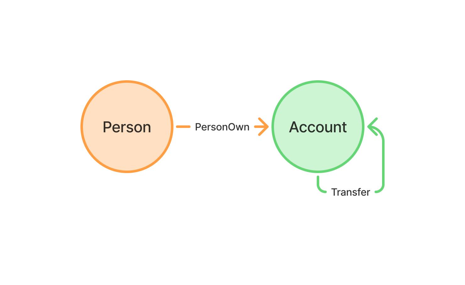
This query gives us a quick overview of the number of entities and connections we're dealing with. As the schema diagram above illustrates, these tables of accounts and transfers already form a graph, a structure made of nodes or vertexes (the entities), connected by edges (representing relations – hint hint – between the entities).

To make our queries more powerful, we'll use the Property Graph model. This is just a formal way of saying we can add descriptive labels, which are general types like Account and Person, as well as specific properties, like accountId and nickname.

If you're thinking this sounds a lot like the relational model, you're exactly right. A Person table is just a collection of nodes with the label Person, and its columns are the properties. This natural mapping is what makes a high-performance relational database like DuckDB a perfect foundation for graph analytics.

Property Graphs in DuckDB

To write our graph queries, we could use DuckDB and the SQL we are familiar with. But let us make life a little simpler for ourselves and leverage DuckDB's rich extension ecosystem. We will be using DuckPGQ, a community extension that adds support to DuckDB's parser for a new visual graph syntax. This new syntax is SQL / Property Graph Queries (SQL/PGQ), which is part of the official SQL:2023 standard. SQL/PGQ is partially inspired by the popular graph query language Cypher.

The DuckPGQ extension started out as a research prototype and is now available as a community extension.

Installing and loading the extension is as simple as it gets:

INSTALL duckpgq FROM community;
LOAD duckpgq;

In DuckPGQ, the first step is to create the property graph, acting as a layer on top of the tables we have created earlier.

CREATE PROPERTY GRAPH finbench
VERTEX TABLES (
    Person,
    Account
)
EDGE TABLES (
    AccountTransferAccount
        SOURCE KEY (fromId) REFERENCES Account (accountId)
        DESTINATION KEY (toId) REFERENCES Account (accountId)
        LABEL Transfer,
    PersonOwnAccount
        SOURCE KEY (personId) REFERENCES Person (personId)
        DESTINATION KEY (accountId) REFERENCES Account (accountId)
        LABEL PersonOwn
);

During the creation of the property graph, we make a clear distinction between VERTEX tables and EDGE tables. For VERTEX tables, we only have to specify the name of the table. For EDGE tables, a little more work is required since for both the SOURCE and the DESTINATION, we need to specify the column in the edge table that forms the key for the SOURCE or DESTINATION. This is the same principle as defining a FOREIGN KEY constraint, linking our edge table back to the node tables it connects. The LABEL clause gives a clean name to the relationship type. While our table is named AccountTransferAccount, the edges within it represent a Transfer relationship. This is the name we'll use in our graph queries.

Now that we have created our property graph, we are ready to investigate the financial data and uncover its secrets!

Graph Processing

When talking about graph processing in databases, we typically refer to these types of operations:

• Pattern matching, finding a pattern in our data.
• Path-finding, finding a path in our data, potentially of variable length.

Let's see how we can leverage DuckDB and DuckPGQ for these two tasks.

Hunting for Suspicious Activities

As previously mentioned, SQL/PGQ introduces a visual graph syntax to formulate graph patterns more naturally. Now, let's use it to hunt for patterns that might indicate a money laundering scheme.

A common technique used to hide illicit funds is called smurfing. The goal of smurfing is to break down a single large transfer, potentially triggering reporting requirements, into smaller transactions over time.

We can search for this behavior by looking for pairs of accounts with a high number of transactions but a relatively low average amount. Let's set the threshold for the average amount at $50,000 and see if we can find any high-frequency relationships:

SELECT
    fromName,
    count(amount) AS number_of_transactions,
    round(avg(amount), 2) AS avg_amount,
    toName
FROM GRAPH_TABLE (finbench
    MATCH (a:Account)-[t:Transfer]->(a2:Account)
    COLUMNS (a.nickname AS fromName,
             t.amount,
             a2.nickname AS toName
            )
)
GROUP BY ALL
HAVING avg_amount < 50_000
ORDER BY number_of_transactions DESC, avg_amount ASC
LIMIT 5;

Running the query leads us to the following result:

┌───────────────────┬────────────────────────┬────────────┬───────────────────┐
│     fromName      │ number_of_transactions │ avg_amount │      toName       │
│      varchar      │         int64          │   double   │      varchar      │
├───────────────────┼────────────────────────┼────────────┼───────────────────┤
│ Noe Trites        │                      1 │   49365.04 │ Dale Croucher     │
│ Madeleine Bussing │                      1 │   46663.56 │ Delphine Primiano │
│ Bonnie Centeno    │                      1 │   46663.56 │ Maile Boon        │
│ Darci Sheedy      │                      1 │   44856.02 │ Carmella Estelle  │
│ Marguerita Gurne  │                      1 │   44393.68 │ Delphine Primiano │
└───────────────────┴────────────────────────┴────────────┴───────────────────┘

The query worked, but the result does not show any signs of suspicious activity with the number of transactions always being 1. To understand why, let's break down how the query was constructed.

The magic happens inside the FROM clause. The GRAPH_TABLE (finbench ...) function allows us to run a graph query over the property graph we have just created and treat its output like a regular table.

The MATCH (a:Account)-[t:Transfer]->(a2:Account) clause is the core of our pattern. It visually describes what we're looking for: a simple transfer from one account (a:Account) to another (a2:Account). The () denote nodes and the [] denotes the connecting edge with the ASCII-style arrow -> showing the direction of the edge. The COLUMNS(...) clause then acts like a SELECT list for our pattern, pulling out the nickname from the accounts and the amount from the transfer.

The beauty of SQL/PGQ is that the result of this graph pattern match can be seamlessly returned into the standard SQL we already know. We use GROUP BY ALL to aggregate all transfers between the same two people, and our HAVING avg_amount < 50_000 clause filters for the smurfing pattern we defined.

We know our query is correct but also that this simple smurfing pattern is not present in our dataset. This means we must investigate further, using potentially more complex patterns. This leads us to a more powerful feature of graph queries: finding structural patterns that are very difficult to express with traditional SQL JOINs, such as transaction paths.

Finding Paths in the Transactions

Another classical example of possible fraudulent behavior is a cycle of transactions where the money circles back to the person who sent the first transaction in the chain. Writing a SQL query to answer this question is, using the traditional syntax, incredibly difficult. Try it yourself, after first reading this section! We will show the answer in the next section.

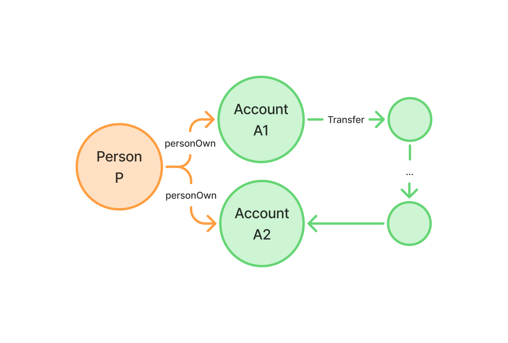
With SQL/PGQ writing queries that involve finding paths has become significantly easier. The diagram above illustrates the query pattern we'll use with the goal of finding a path of one or more transfers between two different accounts (A1 and A2) owned by the same person (P). Remember that persons can own multiple account. With the following query we will try to find cycles between all the accounts that the person with id 125 owns:

FROM GRAPH_TABLE(finbench
    MATCH p = ANY SHORTEST
                  (p:Person)-[o1:PersonOwn]->(a1:Account)
                  -[t:Transfer]->+
                  (a2:Account)<-[o2:PersonOwn]-(p:Person)
WHERE
    p.personId = 125 AND a1.accountId <> a2.accountId
    COLUMNS (
        path_length(p) AS path_length,
        a1.accountId AS start_account,
        a2.accountId AS end_account
    )
)
ORDER BY path_length;

The result shows that there are cycles for this person owning multiple accounts of varying lengths:

┌─────────────┬─────────────────────┬─────────────────────┐
│ path_length │    start_account    │     end_account     │
│    int64    │        int64        │        int64        │
├─────────────┼─────────────────────┼─────────────────────┤
│           8 │ 4753267931712848113 │ 4794926228266025204 │
│           8 │ 4769874955338776819 │ 4794926228266025204 │
│           8 │ 4796615078126289138 │ 4769874955338776819 │
│           9 │ 4753267931712848113 │ 4769874955338776819 │
│           9 │ 4769874955338776819 │ 4753267931712848113 │
│           9 │ 4794926228266025204 │ 4753267931712848113 │
│           9 │ 4796615078126289138 │ 4753267931712848113 │
│           9 │ 4796615078126289138 │ 4794926228266025204 │
│          12 │ 4794926228266025204 │ 4769874955338776819 │
└─────────────┴─────────────────────┴─────────────────────┘

Once again, the magic happens inside the FROM clause where we now create a MATCH that finds ANY SHORTEST path along the given pattern. The first part of the pattern finds all the accounts owned by the Person 125: (p:Person)-[o1:PersonOwn]->(a1:Account). In the second part the path-finding occurs. Take special note of the +, which indicates that for the pattern (a1:Account)-[t:Transfer]->+(a2:Account) the two nodes (a1) and (a2) do not necessarily need to be connected. With the +, we indicate there must be one or more Transfers between these two accounts, with no upper bound set. Finally, to tie it all up, we take the destination account and check whether it is owned by the same person p.

The results confirm our suspicions. Our query found multiple non-obvious paths between the accounts owned by Person 125, with path lengths ranging from 8 to 12 transfers.

Each row represents a hidden chain of transactions connecting two of the person's accounts. More interestingly, we can see clear cyclical patterns. For instance, the query found a 9-step path from account 4753267931712848113 to 4769874955338776819, and another 9-step path flowing in the opposite direction. This suggests a sophisticated and intentional effort to move money between accounts, a strong indicator that warrants further investigation.

Doing it the Old-Fashioned Way

Earlier, we challenged you to think about how you would find these ownership cycles using traditional SQL. As promised, here is the answer.

Before we dive into the query, there are two important notes to keep in mind when comparing it to the SQL/PGQ version:

1. Performance Safeguard: The query requires a manual upper bound on the path length (ps.depth < 11) to prevent infinite recursion and potentially quadratic runtimes on dense graphs. The SQL/PGQ ->+ syntax does not require this.

2. Path Length Difference: You'll notice the path_length in this query's result is two hops shorter than the result from DuckPGQ. This is because this query only counts the Transfer edges, whereas the DuckPGQ query also includes the two PersonOwn edges in its path calculation.

With that in mind, here is the traditional recursive CTE to find the shortest path between any two accounts owned by the same person:

WITH RECURSIVE
    owned_accounts AS (
        SELECT accountId
        FROM PersonOwnAccount
        WHERE personId = 125
    ),
    path_search(start_node, end_node, path, depth) AS (
        -- Base case: a direct transfer from one of the person's accounts
        SELECT
            fromId,
            toId,
            [fromId, toId],
            1
        FROM
            accounttransferaccount
        WHERE
            fromId IN (SELECT accountId FROM owned_accounts)
        UNION ALL
        -- Recursive step: find the next transfer in the path
        SELECT
            ps.start_node,
            t.toId,
            list_append(ps.path, t.toId),
            ps.depth + 1
        FROM path_search ps
        JOIN accounttransferaccount t ON ps.end_node = t.fromId
        WHERE
            t.toId NOT IN (SELECT unnest(ps.path)) AND ps.depth < 11
    )
SELECT distinct start_node, end_node, min(depth) AS path_length
FROM path_search
WHERE end_node IN (SELECT accountId FROM owned_accounts)
  AND start_node <> end_node
GROUP BY ALL
ORDER BY path_length;

As you can see, the logic requires a WITH RECURSIVE clause, manual path tracking in a list, and explicit cycle detection. This is exactly the kind of verbose and complex query that the visual syntax of SQL/PGQ is designed to eliminate.

Wrapping Up

We began this post with a simple goal: to see if we could use DuckDB to hunt for the complex patterns and hidden paths typical of graph analysis. After diving into the Financial Benchmark dataset, the conclusion is clear: you can.

The key takeaway is the drastic improvement in usability. We saw how the visual syntax of SQL/PGQ, enabled by the DuckPGQ extension, transformed a sophisticated "ownership cycle" query from a monstrous recursive CTE into a few readable lines of code. This is exactly the kind of expressive power needed for real-world analytical tasks. For more information and complete documentation on DuckPGQ, be sure to visit its official website: duckpgq.org.

Just as importantly, this entire investigation was performed directly within DuckDB. By leveraging the extension ecosystem, we tapped into the power of graph queries without ever needing to export our data or manage a separate, specialized system. Everything runs on top of DuckDB's high-performance vectorized engine, right where the data lives.

For powerful, analytical graph queries, DuckDB isn't just a viable alternative, it's a powerful, natural solution. The next time you think about analyzing connections in your data, remember that the tools you need are just an INSTALL away.