Basic Feature Engineering with DuckDB
TL;DR: In this post, we show how to perform essential machine learning data preprocessing tasks, like missing value imputation, categorical encoding, and feature scaling, directly in DuckDB using SQL. This approach not only simplifies workflows, but also takes advantage of DuckDB’s high-performance, in-process execution engine for fast, efficient data preparation.
Introduction
Data preprocessing is a necessary step in any machine learning workflow, affecting both the model’s effectiveness and the ease of maintenance. While scikit-learn is commonly used for preprocessing due to its integration with the broader Python ecosystem, DuckDB offers a practical alternative by enabling SQL-based data transformations within Python. Its declarative syntax supports modular workflows, making preprocessing steps easier to isolate, inspect, and debug. In addition, DuckDB’s support for efficient querying of columnar data formats and its ability to persist preprocessing logic as SQL scripts contribute to more reproducible and transparent pipelines.
Data Preparation
We will be working with a synthetic financial transactions dataset from Kaggle, which contains generic information used for fraud detection in financial transactions.
CREATE TABLE financial_trx AS
    FROM read_csv('https://blobs.duckdb.org/data/financial_fraud_detection_dataset.csv');
We start by analyzing the data by executing SUMMARIZE:
FROM (SUMMARIZE financial_trx)
SELECT
    column_name,
    column_type,
    count,
    null_percentage,
    min;
┌─────────────────────────────┬─────────────┬─────────┬─────────────────┬────────────────────────────┐
│         column_name         │ column_type │  count  │ null_percentage │            min             │
│           varchar           │   varchar   │  int64  │  decimal(9,2)   │          varchar           │
├─────────────────────────────┼─────────────┼─────────┼─────────────────┼────────────────────────────┤
│ transaction_id              │ VARCHAR     │ 5000000 │            0.00 │ T100000                    │
│ timestamp                   │ TIMESTAMP   │ 5000000 │            0.00 │ 2023-01-01 00:09:26.241974 │
│ sender_account              │ VARCHAR     │ 5000000 │            0.00 │ ACC100000                  │
│ receiver_account            │ VARCHAR     │ 5000000 │            0.00 │ ACC100000                  │
│ amount                      │ DOUBLE      │ 5000000 │            0.00 │ 0.01                       │
│ transaction_type            │ VARCHAR     │ 5000000 │            0.00 │ deposit                    │
│ merchant_category           │ VARCHAR     │ 5000000 │            0.00 │ entertainment              │
│ location                    │ VARCHAR     │ 5000000 │            0.00 │ Berlin                     │
│ device_used                 │ VARCHAR     │ 5000000 │            0.00 │ atm                        │
│ is_fraud                    │ BOOLEAN     │ 5000000 │            0.00 │ false                      │
│ fraud_type                  │ VARCHAR     │ 5000000 │           96.41 │ card_not_present           │
│ time_since_last_transaction │ DOUBLE      │ 5000000 │           17.93 │ -8777.814181944444         │
│ spending_deviation_score    │ DOUBLE      │ 5000000 │            0.00 │ -5.26                      │
│ velocity_score              │ BIGINT      │ 5000000 │            0.00 │ 1                          │
│ geo_anomaly_score           │ DOUBLE      │ 5000000 │            0.00 │ 0.0                        │
│ payment_channel             │ VARCHAR     │ 5000000 │            0.00 │ ACH                        │
│ ip_address                  │ VARCHAR     │ 5000000 │            0.00 │ 0.0.102.150                │
│ device_hash                 │ VARCHAR     │ 5000000 │            0.00 │ D1000002                   │
├─────────────────────────────┴─────────────┴─────────┴─────────────────┴────────────────────────────┤
│ 18 rows                                                                                  5 columns │
└────────────────────────────────────────────────────────────────────────────────────────────────────┘
Feature Encoding
From the above data stats, we see that there are a few category columns, such as transaction_type, merchant_category and payment_channel. Because most machine learning models expect numerical inputs, this type of data is converted to a numerical representation. This process is called encoding, and it can be done in multiple ways. In the following, we showcase a few common encoding techniques in SQL.
In this post, we use several of DuckDB's “friendly SQL” features, including the
FROM-first syntax and prefix aliases.
One-Hot Encoding
When applying one-hot encoding over a category column, each distinct value is transposed into its own column and it gets the value 1 for match and 0 for not a match:
FROM financial_trx
SELECT DISTINCT
    transaction_type,
    deposit_onehot: (transaction_type = 'deposit')::INT,
    payment_onehot: (transaction_type = 'payment')::INT,
    transfer_onehot: (transaction_type = 'transfer')::INT,
    withdrawal_onehot: (transaction_type = 'withdrawal')::INT
ORDER BY transaction_type;
┌──────────────────┬────────────────┬────────────────┬─────────────────┬───────────────────┐
│ transaction_type │ deposit_onehot │ payment_onehot │ transfer_onehot │ withdrawal_onehot │
│     varchar      │     int32      │     int32      │      int32      │       int32       │
├──────────────────┼────────────────┼────────────────┼─────────────────┼───────────────────┤
│ deposit          │              1 │              0 │               0 │                 0 │
│ payment          │              0 │              1 │               0 │                 0 │
│ transfer         │              0 │              0 │               1 │                 0 │
│ withdrawal       │              0 │              0 │               0 │                 1 │
└──────────────────┴────────────────┴────────────────┴─────────────────┴───────────────────┘
Another way to one-hot encode is by using the PIVOT statement:
PIVOT financial_trx
ON transaction_type
USING coalesce(max(transaction_type = transaction_type)::INT, 0) AS onehot
GROUP BY transaction_type;
In the above statement we:
- pivot on the category column,
transaction_type; - the pivot condition is for
transaction_typeto match each value of itself; - we convert boolean to integer and apply max over the match;
- we alias the transposed columns as the value of
transaction_typesuffixed by_onehot.
If there are more category columns to be one-hot encoded then PIVOT can be used in subqueries or WITH clauses:
WITH onehot_trx_type AS (
    PIVOT financial_trx
    ON transaction_type
    USING coalesce(max(transaction_type = transaction_type)::INT, 0) AS onehot
    GROUP BY transaction_type
), onehot_payment_channel AS (
    PIVOT financial_trx
    ON payment_channel
    USING coalesce(max(payment_channel = payment_channel)::INT, 0) AS onehot
    GROUP BY payment_channel
)
SELECT
    financial_trx.*,
    onehot_trx_type.* LIKE '%\_onehot' ESCAPE '\',
    onehot_payment_channel.* LIKE '%\_onehot' ESCAPE '\'
FROM financial_trx
INNER JOIN onehot_trx_type USING (transaction_type)
INNER JOIN onehot_payment_channel USING (payment_channel);
In the above query we are retrieving all “onehot”-suffixed columns by using the
LIKEoperator on column names.
Ordinal Encoding
Ordinal encoding assigns a unique identifier to each categorical value and it is usually applied when there is a certain hierarchy in the categorical values. For example, we can assign the identifier with the row_number function and ordering by the transaction type:
WITH trx_type_ordinal_encoded AS (
    SELECT
        transaction_type,
        trx_type_oe: row_number() OVER (ORDER BY transaction_type) - 1
    FROM (
        SELECT DISTINCT transaction_type
        FROM financial_trx
    )
)
SELECT
    transaction_type,
    trx_type_oe,
    number_trx: count(*)
FROM financial_trx
INNER JOIN trx_type_ordinal_encoded USING (transaction_type)
GROUP BY ALL
ORDER BY trx_type_oe;
┌──────────────────┬─────────────┬────────────┐
│ transaction_type │ trx_type_oe │ number_trx │
│     varchar      │    int64    │   int64    │
├──────────────────┼─────────────┼────────────┤
│ deposit          │           0 │    1250593 │
│ payment          │           1 │    1250438 │
│ transfer         │           2 │    1250334 │
│ withdrawal       │           3 │    1248635 │
└──────────────────┴─────────────┴────────────┘
Label Encoding
Similarly to ordinal encoding, label encoding assigns a unique identifier, but it does not take order into account and it is, usually, applied to output data:
WITH trx_type_label_encoded AS (
    SELECT
        transaction_type,
        trx_type_le: row_number() OVER () - 1
    FROM (
        SELECT DISTINCT transaction_type
        FROM financial_trx
    )
)
SELECT
    transaction_type,
    trx_type_le,
    number_trx: count(*)
FROM financial_trx
INNER JOIN trx_type_label_encoded USING (transaction_type)
GROUP BY ALL
ORDER BY trx_type_le;
┌──────────────────┬─────────────┬────────────┐
│ transaction_type │ trx_type_le │ number_trx │
│     varchar      │    int64    │   int64    │
├──────────────────┼─────────────┼────────────┤
│ deposit          │           0 │    1250593 │
│ withdrawal       │           1 │    1248635 │
│ payment          │           2 │    1250438 │
│ transfer         │           3 │    1250334 │
└──────────────────┴─────────────┴────────────┘
Another way to achieve the above is by using list functions, such as array_agg, to create an array with the distinct values, and list_position to extract the position of each value in the array:
WITH trx_ref AS (
    SELECT trx_type_values: array_agg(DISTINCT transaction_type)
    FROM financial_trx
)
SELECT
    transaction_type,
    trx_type_le: list_position(trx_type_values, transaction_type) - 1,
    number_trx: count(*)
FROM
    financial_trx,
    trx_ref
GROUP BY ALL
ORDER BY trx_type_le;
┌──────────────────┬─────────────┬────────────┐
│ transaction_type │ trx_type_le │ number_trx │
│     varchar      │    int32    │   int64    │
├──────────────────┼─────────────┼────────────┤
│ payment          │           0 │    1250438 │
│ deposit          │           1 │    1250593 │
│ transfer         │           2 │    1250334 │
│ withdrawal       │           3 │    1248635 │
└──────────────────┴─────────────┴────────────┘
The above queries are non-deterministic, therefore a sort or storing the data in a reference table might be required for incremental processing.
Feature Scaling
One other common data preprocessing step in machine learning is to scale numerical features, such that the values of different features are brought to a similar range or distribution. Scaling, also known as feature normalization or standardization, involves transforming features so they have comparable magnitudes; typically by rescaling them to a fixed range (like 0 to 1) or adjusting them to have zero mean and unit variance. This process is required because many algorithms rely on distance calculations or gradient updates, which can be skewed if features vary widely in scale.
If encoding is performed on the initial raw data (due to the need of knowing the entire categorical values list), scaling requires to split the data into training and testing data sets, in order to avoid data leakage. In DuckDB, we can split the data by sampling it:
SET threads = 1;

CREATE TABLE financial_trx_training AS
FROM financial_trx
USING SAMPLE 80 PERCENT (reservoir, 256);

SET threads = 8;

CREATE TABLE financial_trx_testing AS
FROM financial_trx
ANTI JOIN financial_trx_training USING (transaction_id);
We configure DuckDB to use a single-thread during sampling and set a
seedto make sure that the sampling is reproducible. We also apply thereservoirsampling strategy to have exactly 80% of the records in the resulting sample.
Standard Scaling
Standard scaling is a preprocessing technique that transforms numerical features by subtracting the mean and dividing by the standard deviation, so that each feature has a mean of 0 and a standard deviation of 1.
For example, to standard scaling velocity_score, we can run:
WITH scaling_params AS (
    SELECT
        avg_velocity_score: avg(velocity_score),
        stddev_pop_velocity_score: stddev_pop(velocity_score)
    FROM financial_trx_training
)
SELECT
    ss_velocity_score: (velocity_score - avg_velocity_score) /
        stddev_pop_velocity_score
FROM
    financial_trx_testing,
    scaling_params;
The above query can be greatly simplified by using DuckDB macros. With scalar macros, we can create a function for the standard scaler transformation:
CREATE OR REPLACE MACRO standard_scaler(val, avg_val, std_val) AS
    (val - avg_val) / std_val;
With table macros, we can create a function to return the scaling parameters required by the standard scaler macro:
CREATE OR REPLACE MACRO scaling_params(table_name, column_list) AS TABLE
    FROM query_table(table_name)
    SELECT
        "avg_\0": avg(columns(column_list)),
        "std_\0": stddev_pop(columns(column_list));
In the above macro definition:
- any table can be provided as input parameter and queried due to
query_table; - we apply aggregate functions over the list of columns provided as input parameter, by using column expressions;
- we generate the aggregate alias by using the original column name via the
\0in the alias definition.
We can now calculate the standard scaling as follows:
SELECT
    ss_velocity_score: standard_scaler(
        velocity_score,
        avg_velocity_score,
        std_velocity_score
    ),
    ss_spending_deviation_score: standard_scaler(
        spending_deviation_score,
        avg_spending_deviation_score,
        std_spending_deviation_score
    )
FROM financial_trx_testing,
    scaling_params(
        'financial_trx_training',
        ['velocity_score', 'spending_deviation_score']
    );
Min-Max Scaling
Min-Max scaling is a normalization technique that transforms features to a fixed range, typically 0 to 1, by subtracting the minimum value and dividing by the range (max − min). This preserves the shape of the original distribution while ensuring all values are on the same scale.
In order to min-max scale our feature, we expand the scaling_params macro with the calculation of min and max over the input column list:
CREATE OR REPLACE MACRO scaling_params(table_name, column_list) AS TABLE
    FROM query_table(table_name)
    SELECT
        "avg_\0": avg(columns(column_list)),
        "std_\0": stddev_pop(columns(column_list)),
        "min_\0": min(columns(column_list)),
        "max_\0": max(columns(column_list));
We then define a macro definition for the min-max calculation:
CREATE OR REPLACE MACRO min_max_scaler(val, min_val, max_val) AS
(val - min_val) / nullif(max_val - min_val, 0);
Finally, we extract the values:
SELECT
    min_max_velocity_score: min_max_scaler(
        velocity_score,
        min_velocity_score,
        max_velocity_score
    ),
    min_max_spending_deviation_score: min_max_scaler(
        spending_deviation_score,
        min_spending_deviation_score,
        max_spending_deviation_score
    )
FROM financial_trx_testing,
    scaling_params(
        'financial_trx_training',
        ['velocity_score', 'spending_deviation_score']
    );
Robust Scaling
Robust scaling is a data normalization technique that transforms numerical features by subtracting the median and dividing by the interquartile range (IQR). Unlike standard scaling, which uses the mean and standard deviation, robust scaling reduces the influence of outliers by focusing on the middle 50% of the data. This makes it well-suited for datasets with skewed distributions or extreme values.
In DuckDB, we can calculate the quantile ranges with the quantile_cont statistical aggregate:
CREATE OR REPLACE MACRO scaling_params(table_name, column_list) AS TABLE
    FROM query_table(table_name)
    SELECT
        "avg_\0": avg(columns(column_list)),
        "std_\0": stddev_pop(columns(column_list)),
        "min_\0": min(columns(column_list)),
        "max_\0": max(columns(column_list)),
        "q25_\0": quantile_cont(columns(column_list), 0.25),
        "q50_\0": quantile_cont(columns(column_list), 0.50),
        "q75_\0": quantile_cont(columns(column_list), 0.75);
We define the scalar macro for the robust scaling calculation:
CREATE OR REPLACE MACRO robust_scaler(val, q25_val, q50_val, q75_val) AS
    (val - q50_val) / nullif(q75_val - q25_val, 0);
And, similarly with the other scaling transformations, we call it in SQL directly:
SELECT
    rs_velocity_score: robust_scaler(
        velocity_score,
        q25_velocity_score,
        q50_velocity_score,
        q75_velocity_score
    ),
    rs_spending_deviation_score: robust_scaler(
        spending_deviation_score,
        q25_spending_deviation_score,
        q50_spending_deviation_score,
        q75_spending_deviation_score
    )
FROM financial_trx_testing,
    scaling_params(
        'financial_trx_training',
        ['velocity_score', 'spending_deviation_score']
    );
Handling Missing Values
It often happens that our input data is incomplete, i.e., it has missing data. Depending on the use case, such data is excluded, used as it is or filled with a constant value. In DuckDB we can use the coalesce function in order to retrieve the value of the column or a default value, if the column is NULL.
Some common techniques are to:
- replace missing values with a constant;
- replace missing values with the average;
- replace missing values with the median.
We extend the scaling_params macro by adding the median calculation:
CREATE OR REPLACE MACRO scaling_params(table_name, column_list) AS TABLE
    FROM query_table(table_name)
    SELECT
        "avg_\0": avg(columns(column_list)),
        "std_\0": stddev_pop(columns(column_list)),
        "min_\0": min(columns(column_list)),
        "max_\0": max(columns(column_list)),
        "q25_\0": quantile_cont(columns(column_list), 0.25),
        "q50_\0": quantile_cont(columns(column_list), 0.50),
        "q75_\0": quantile_cont(columns(column_list), 0.75),
        "median_\0": median(columns(column_list));
And we apply coalesce to handle the missing values according to our use-case:
SELECT
    time_since_last_transaction_with_0: coalesce(time_since_last_transaction, 0),
    time_since_last_transaction_with_mean: coalesce(time_since_last_transaction, avg_time_since_last_transaction),
    time_since_last_transaction_with_libraryn: coalesce(time_since_last_transaction, median_time_since_last_transaction)
FROM
    financial_trx_testing,
    scaling_params('financial_trx_training', ['time_since_last_transaction'])
WHERE time_since_last_transaction IS NULL;
Filling missing data should be done before feature scaling.
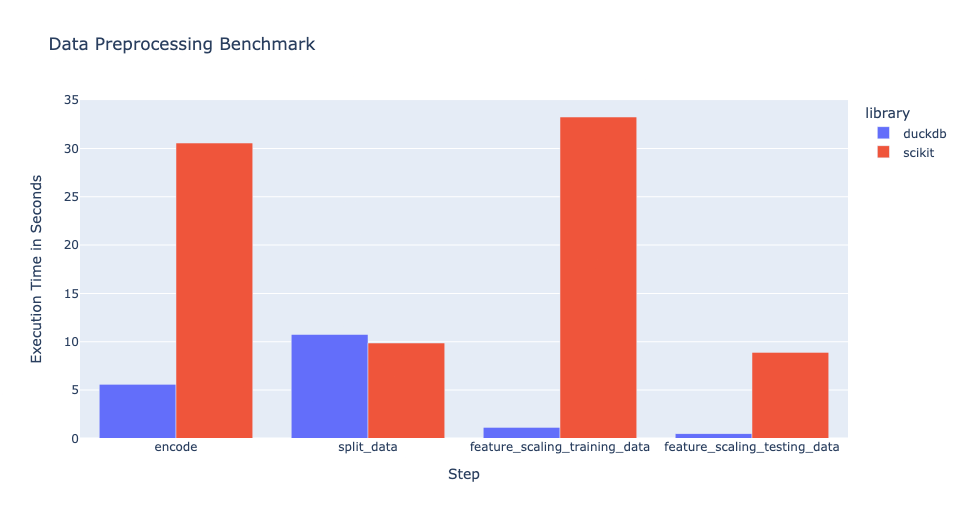
Benchmark
Bringing the above data processing steps together, we have decided to benchmark the execution time against the scikit-learn data preprocessing pipelines.
The code is available in our blog examples repository.
In scikit-learn, data preprocessing is done through transformers and pipelines.
A transformer is a class that implements the fit and transform methods, while a pipeline is a sequence of transformers that are applied to the data in a specific order.
Unless specified otherwise, each step of the pipeline returns, in numpy arrays, only the result of the transformation step.
Because in DuckDB we transform the data through SQL expressions, we can inspect the full data set after each step.
Therefore, in our benchmark, the scikit-learn data preprocessing steps include the following transformations:
- the output of the transformation step is set to
pandas; - all the columns are passed through the transformation step, by setting
remainder='passthrough'.
from sklearn.compose import ColumnTransformer
from sklearn.impute import SimpleImputer
from sklearn.pipeline import Pipeline
from sklearn.preprocessing import StandardScaler, MinMaxScaler, RobustScaler


def scikit_feature_scaling_training_data(x_train):
    impute_missing_data = Pipeline(
        [
            ("imputer", SimpleImputer(strategy="mean")),
            ("scaler", MinMaxScaler(copy=False)),
        ]
    )

    scaling_steps = ColumnTransformer(
        [
            (
                "ss",
                StandardScaler(copy=False),
                ["velocity_score"]
            ),
            (
                "minmax_time_since_last_transaction",
                impute_missing_data,
                ["time_since_last_transaction"],
            ),
            (
                "minmax",
                MinMaxScaler(copy=False),
                ["spending_deviation_score"]
            ),
            (
                "rs",
                RobustScaler(copy=False),
                ["amount"]
            ),
        ],
        remainder="passthrough",
        verbose_feature_names_out=False,
    )

    scaling_steps.set_output(transform="pandas")
    scaling_steps.fit(x_train)

    return scaling_steps, scaling_steps.transform(x_train)
The figure below shows the execution times on a MacBook Pro with 16 GB,
demonstrating that DuckDB offers a significant performance improvement over scikit-learn for the data preprocessing steps.
In the script
reconcile_results.py, the results between the DuckDB andscikit-learnpreprocessing steps are reconciled, demonstrating that both implementations produce the same results.
In the above examples, we demonstrated how to perform data preprocessing with SQL expressions during training.
In practice, the same preprocessing steps must be applied at inference time, such that new data is transformed consistently with the training data.
With scikit-learn, this is achieved by persisting the pipeline alongside the model and applying the pipeline at inference time.
With DuckDB, the equivalent consistency is achieved by persisting the original training data (or the metrics returned by the scaling_params macro, computed during training).
Despite the (transformed) training data being much larger than the model artifacts, versioning the data and features calculated at training time is a common practice, which ensures model traceability and reproducibility.
For efficient (training) data management, one can leverage solutions that provide time travel, such as DuckLake.
Conclusion
In this article we showed how DuckDB offers a performant and SQL-native approach to data preprocessing for machine learning workflows. By handling tasks such as missing value imputation, categorical encoding, and feature scaling directly within the database engine, one can eliminate unnecessary data movement, during training, and reduce preprocessing latency.

