Driving CSV Performance: Benchmarking DuckDB with the NYC Taxi Dataset

TL;DR: DuckDB's benchmark suite now includes the NYC Taxi Benchmark. We explain how our CSV reader performs on the Taxi Dataset and provide steps to reproduce the benchmark.
The NYC taxi dataset is a collection of many years of taxi rides that occurred in New York City. It is a very influential dataset, used for database benchmarks, machine learning, data visualization, and more.
In 2022, the data provider has decided to distribute the dataset as a series of Parquet files instead of CSV files. Performance-wise, this is a wise choice, as Parquet files are much smaller than CSV files, and their native columnar format allows for fast execution directly on them. However, this change hinders the number of systems that can natively load the files.
In the “Billion Taxi Rides in Redshift” blog post, a new database benchmark is proposed to evaluate the performance of aggregations over the taxi dataset. The dataset is also joined and denormalized with other datasets that contain information about the weather, cab types, and pickup/dropoff locations. It is then stored as multiple compressed, gzipped CSV files, each containing 20 million rows.
The Taxi Data Set as CSV Files
Since DuckDB is well-known for its CSV reader performance, we were intrigued to explore whether the loading process of this benchmark could help us identify new performance bottlenecks in our CSV loader. This curiosity led us on a journey to generate these datasets and analyze their performance in DuckDB. According to the recent study conducted on the AWS RedShift fleet, CSV files are the most used external source data type in S3, and 99% of them are gzipped. Therefore, the fact that the proposed benchmark also used split gzipped files caught my attention.
In this blog post, we'll guide you through how to run this benchmark in DuckDB and discuss some lessons learned and future ideas for our CSV Reader. The dataset used in this benchmark is publicly available. The dataset is partitioned and distributed as a collection of 65 gzipped CSV files, each containing 20 million rows and totaling up to 1.8 GB per file. The total dataset is 111 GB compressed and 518 GB uncompressed. We also provide more details on how we generated this dataset and highlight the differences between the dataset we distribute and the original one described in the “Billion Taxi Rides in Redshift” blog post.
Reproducing the Benchmark
Doing fair benchmarking is a difficult problem, especially when the data, queries, and results used for the benchmark are not easy to access and run. We have made the benchmark discussed in this blog post easy to run by providing scripts available in the taxi-benchmark GitHub repository.
This repository contains three main Python scripts:
generate_prepare_data.py: Downloads all necessary files and prepares them for the benchmark.benchmark.py: Runs the benchmark and performs result verification.analyse.py: Analyzes the benchmark results and produces some of the insights discussed in this blog post.
The benchmark is not intended to be flawless – no benchmark is. However, we believe that sharing these scripts is a positive step, and we welcome any contributions to make them cleaner and more efficient.
The repository also includes a README file with detailed instructions on how to use it. This repository will serve as the foundation for the experiments conducted in this blog post.
Preparing the Dataset
To start, you first need to download and prepare the files by executing python generate_prepare_data.py. This will download all 65 files to the ./data folder. Additionally, the files will be uncompressed and combined into a single large file.
As a result, the ./data folder will have 65 gzipped CSV files (i.e., from trips_xaa.csv.gz to trips_xcm.csv.gz) and a single large uncompressed CSV file containing the full data (i.e., decompressed.csv).
Our benchmark then run in two different settings:
- Over 65 compressed files.
- Over a single uncompressed file.
Once the files have been prepared, you can run the benchmark by running python benchmark.py.
Loading
The loading phase of the benchmark runs six times for each benchmark setting. From the first five runs, we take the median loading time. During the sixth run, we collect resource usage data (e.g., CPU usage and disk reads/writes).
Loading is performed using an in-memory DuckDB instance, meaning the data is not persisted to DuckDB storage and only exists while the connection is active. This is important to note because, as the dataset does not fit in memory and is spilled into a temporary space on disk. The decision to not persist the data has a substantial impact on performance: it makes loading the dataset significantly faster, while querying it will be somewhat slower as DuckDB will use an uncompressed representation. We made this choice for the benchmark since our primary focus is on testing the CSV loader rather than the queries.
Our table schema is defined in schema.sql.
schema.sql.
CREATE TABLE trips (
    trip_id                 BIGINT,
    vendor_id               VARCHAR,
    pickup_datetime         TIMESTAMP,
    dropoff_datetime        TIMESTAMP,
    store_and_fwd_flag      VARCHAR,
    rate_code_id            BIGINT,
    pickup_longitude        DOUBLE,
    pickup_latitude         DOUBLE,
    dropoff_longitude       DOUBLE,
    dropoff_latitude        DOUBLE,
    passenger_count         BIGINT,
    trip_distance           DOUBLE,
    fare_amount             DOUBLE,
    extra                   DOUBLE,
    mta_tax                 DOUBLE,
    tip_amount              DOUBLE,
    tolls_amount            DOUBLE,
    ehail_fee               DOUBLE,
    improvement_surcharge   DOUBLE,
    total_amount            DOUBLE,
    payment_type            VARCHAR,
    trip_type               VARCHAR,
    pickup                  VARCHAR,
    dropoff                 VARCHAR,
    cab_type                VARCHAR,
    precipitation           BIGINT,
    snow_depth              BIGINT,
    snowfall                BIGINT,
    max_temperature         BIGINT,
    min_temperature         BIGINT,
    average_wind_speed      BIGINT,
    pickup_nyct2010_gid     BIGINT,
    pickup_ctlabel          VARCHAR,
    pickup_borocode         BIGINT,
    pickup_boroname         VARCHAR,
    pickup_ct2010           VARCHAR,
    pickup_boroct2010       BIGINT,
    pickup_cdeligibil       VARCHAR,
    pickup_ntacode          VARCHAR,
    pickup_ntaname          VARCHAR,
    pickup_puma             VARCHAR,
    dropoff_nyct2010_gid    BIGINT,
    dropoff_ctlabel         VARCHAR,
    dropoff_borocode        BIGINT,
    dropoff_boroname        VARCHAR,
    dropoff_ct2010          VARCHAR,
    dropoff_boroct2010      BIGINT,
    dropoff_cdeligibil      VARCHAR,
    dropoff_ntacode         VARCHAR,
    dropoff_ntaname         VARCHAR,
    dropoff_puma            VARCHAR);
The loader for the 65 files uses the following query:
COPY trips FROM 'data/trips_*.csv.gz' (HEADER false);
The loader for the single uncompressed file uses this query:
COPY trips FROM 'data/decompressed.csv' (HEADER false);
Querying
After loading, the benchmark script will run each of the benchmark queries five times to measure their execution time. It is also important to note that the results of the queries are validated against their corresponding answers. This allows us to verify the correctness of the benchmark. Additionally, the queries are identical to those used in the original “Billion Taxi Rides” benchmark.
Results
Loading Time
Although we are talking about many rows of a CSV file with 51 columns, DuckDB can ingest them rather fast.
Note that, by default, DuckDB preserves the insertion order of the data, which negatively impacts performance. In the following results, all datasets have been loaded with this option set to false.
SET preserve_insertion_order = false;
All experiments were run on my Apple M1 Max with 64 GB of RAM, and we compare the loading times for a single uncompressed CSV file, and the 65 compressed CSV files.
| Name | Time (min) | Avg deviation of CPU usage from 100% |
|---|---|---|
| Single File – Uncompressed | 11:52 | 31.57 |
| Multiple Files – Compressed | 13:52 | 27.13 |
Unsurprisingly, loading data from multiple compressed files is more CPU-efficient than loading from a single uncompressed file. This is evident from the lower average deviation in CPU usage for multiple compressed files, indicating fewer wasted CPU cycles. There are two main reasons for this: (1) The compressed files are approximately eight times smaller than the uncompressed file, drastically reducing the amount of data that needs to be loaded from disk and, consequently, minimizing CPU stalls while waiting for data to be processed. (2) It is much easier to parallelize the loading of multiple files than a single file, as each thread can handle on a single file.
The difference in CPU efficiency is also reflected in execution times: reading from a single uncompressed file is 2 minutes faster than reading from multiple compressed files. The reason for this lies in our decompression algorithm, which is admittedly not optimally designed. Reading a compressed file involves three tasks: (1) loading data from disk into a compressed buffer, (2) decompressing that data into a decompressed buffer, and (3) processing the decompressed buffer. In our current implementation, tasks 1 and 2 are combined into a single operation, meaning we cannot continue reading until the current buffer is fully decompressed, resulting in idle cycles.
Under the Hood
We can also see what happens under the hood to verify our conclusion regarding the loading time.
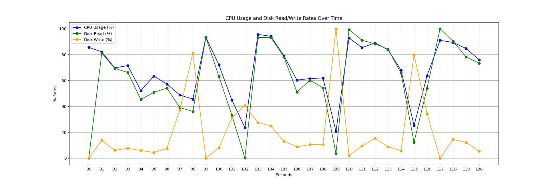
In the figure below, you can see a snapshot of CPU and disk utilization for the “Single File – Uncompressed” run. We observe that achieving 100% CPU utilization is challenging, and we frequently experience stalls due to data writes to disk, as we are creating a table from a dataset that does not fit into our memory. Another key point is that CPU utilization is closely tied to disk reads, indicating that our threads often wait for data before processing it. Implementing async IO for the CSV Reader/Writer could significantly improve performance for parallel processing, as a single thread could handle most of our disk I/O without negatively affecting CPU utilization.
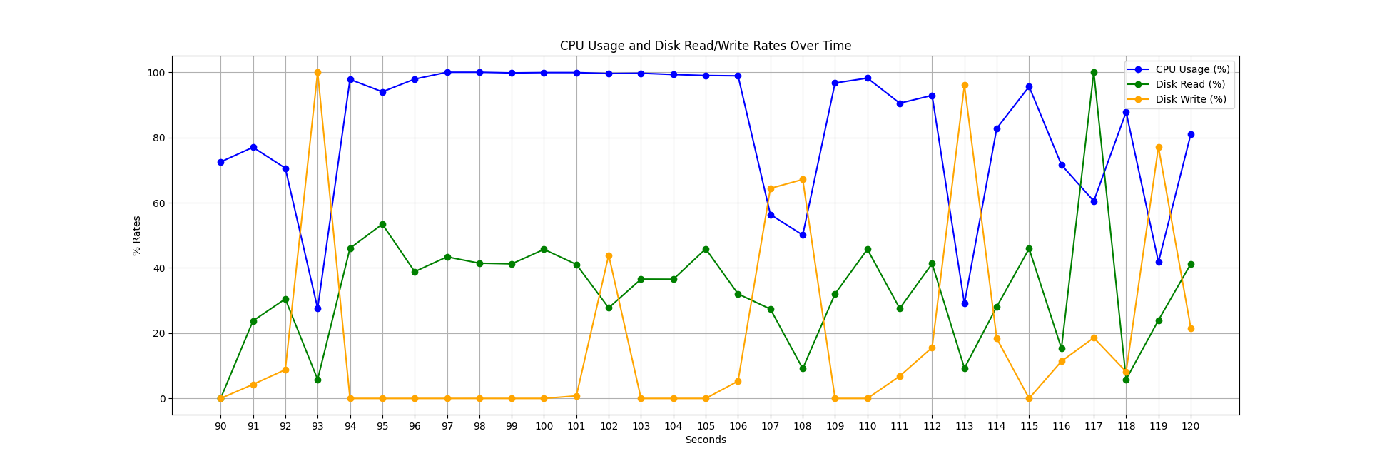
Below, you can see a similar snapshot for loading the 65 compressed files. We frequently encounter stalls during data writes; however, CPU utilization is significantly better because we wait less time for the data to load (remember, the data is approximately 8 times smaller than in the uncompressed case). In this scenario, parallelization is also much easier. Like in the uncompressed case, these gaps in CPU utilization could be mitigated by async I/O, with the addition of a decomposed decompression algorithm.
Query Times
For completeness, we also provide the results of the four queries on a MacBook Pro with an M1 Pro CPU. This comparison demonstrates the time differences between querying a database that does not fit in memory using a purely in-memory connection (i.e., without storage) versus one where the data is first loaded and persisted in the database.
| Name | Time – without storage (s) | Time – with storage (s) |
|---|---|---|
| Q 01 | 2.45 | 1.45 |
| Q 02 | 3.89 | 0.80 |
| Q 03 | 5.21 | 2.20 |
| Q 04 | 11.2 | 3.12 |
The main difference between these times is that when DuckDB uses a storage file, the data is highly compressed, resulting in much faster access when querying the dataset.
In contrast, when we do not use persistent storage, our in-memory database temporarily stores data in an uncompressed .tmp file to allow for memory overflow, which increases disk I/O and leads to slower query results. This observation raises a potential area for exploration: determining whether applying compression to temporary data would be beneficial.
How This Dataset Was Generated
The original blog post generated the dataset using CSV files distributed by the NYC Taxi and Limousine Commission. Originally, these files included precise latitude and longitude coordinates for pickups and drop-offs. However, starting in mid-2016, these precise coordinates were anonymized using pickup and drop-off geometry objects to address privacy concerns. (There are even stories of broken marriages resulting from checking the actual destinations of taxis.) Furthermore, in recent years, the TLC decided to redistribute the data as Parquet files and to fully anonymize these data points, including data prior to mid-2016.
This is a problem, as the dataset from the “Billion Taxi Rides in Redshift” blog post relies on having this detailed information. Let's take the following snippet of the data:
649084905,VTS,2012-08-31 22:00:00,2012-08-31 22:07:00,0,1,-73.993908,40.741383000000006,-73.989915,40.75273800000001,1,1.32,6.1,0.5,0.5,0,0,0,0,7.1,CSH,0,0101000020E6100000E6CE4C309C7F52C0BA675DA3E55E4440,0101000020E610000078B471C45A7F52C06D3A02B859604440,yellow,0.00,0.0,0.0,91,69,4.70,142,54,1,Manhattan,005400,1005400,I,MN13,Hudson Yards-Chelsea-Flatiron-Union Square,3807,132,109,1,Manhattan,010900,1010900,I,MN17,Midtown-Midtown South,3807
We see precise longitude and latitude data points: -73.993908, 40.741383000000006, -73.989915, 40.75273800000001, along with a PostGIS Geometry hex blob created from this longitude and latitude information: 0101000020E6100000E6CE4C309C7F52C0BA675DA3E55E4440, 0101000020E610000078B471C45A7F52C06D3A02B859604440 (generated as ST_SetSRID(ST_Point(longitude, latitude), 4326)).
Since this information is essential to the dataset, producing files as described in the “Billion Taxi Rides in Redshift” blog post is no longer feasible due to the missing detailed location data. However, the internet never forgets. Hence, we located instances of the original dataset distributed by various sources, such as [1], [2], and [3]. Using these sources, we combined the original CSV files with weather information from the scripts referenced in the “Billion Taxi Rides in Redshift” blog post.
How Does This Dataset Differ from the Original One?
There are two significant differences between the dataset we distribute and the one from the “Billion Taxi Rides in Redshift” blog post:
- Our dataset includes data up to the last date that longitude and latitude information was available (June 30, 2016), whereas the original post only included data up to the end of 2015 (understandable, as the post was written in February 2016).
- We also included Uber trips, which were excluded from the original post.
If you wish to run the benchmark with a dataset as close to the original as possible, you can generate a new table by filtering out the additional data. For example:
CREATE TABLE trips_og AS
    FROM trips
    WHERE pickup_datetime < '2016-01-01'
      AND cab_type != 'uber';
Conclusion
In this blog post, we discussed how to run the taxi benchmark on DuckDB, and we've made all scripts available so you can benchmark your preferred system as well. We also demonstrated how this highly relevant benchmark can be used to evaluate our operators and gain insights into areas for further improvement.

