Persistent Storage of Adaptive Radix Trees (ART) in DuckDB

TL;DR: DuckDB uses Adaptive Radix Tree (ART) Indexes to enforce constraints and to speed up query filters. Up to this point, indexes were not persisted, causing issues like loss of indexing information and high reload times for tables with data constraints. We now persist ART Indexes to disk, drastically diminishing database loading times (up to orders of magnitude), and we no longer lose track of existing indexes. This blog post contains a deep dive into the implementation of ART storage, benchmarks, and future work. Finally, to better understand how our indexes are used, I'm asking you to answer the following survey. It will guide us when defining our future roadmap.

DuckDB uses ART Indexes to keep primary key (PK), foreign key (FK), and unique constraints. They also speed up point-queries, range queries (with high selectivity), and joins. Before the bleeding edge version (or V0.4.1, depending on when you are reading this post), DuckDB did not persist ART indexes on disk. When storing a database file, only the information about existing PKs and FKs would be stored, with all other indexes being transient and non-existing when restarting the database. For PKs and FKs, they would be fully reconstructed when reloading the database, creating the inconvenience of high-loading times.
A lot of scientific work has been published regarding ART Indexes, most notably on synchronization, cache-efficiency, and evaluation. However, up to this point, no public work exists on serializing and buffer managing an ART Tree. Some say that Hyper, the database in Tableau, persists ART indexes, but again, there is no public information on how that is done.
This blog post will describe how DuckDB stores and loads ART indexes. In particular, how the index is lazily loaded (i.e., an ART node is only loaded into memory when necessary). In the ART Index Section, we go through what an ART Index is, how it works, and some examples. In the ART in DuckDB Section, we explain why we decided to use an ART index in DuckDB where it is used and discuss the problems of not persisting ART indexes. In the ART Storage Section, we explain how we serialize and buffer manage ART Indexes in DuckDB. In the Benchmarks Section, we compare DuckDB v0.4.0 (before ART Storage) with the bleeding edge version of DuckDB. We demonstrate the difference in the loading costs of PKs and FKs in both versions and the differences between lazily loading an ART index and accessing a fully loaded ART Index. Finally, in the Road Map section, we discuss the drawbacks of our current implementations and the plans on the list of ART index goodies for the future.
ART Index
Adaptive Radix Trees are, in essence, tries that apply vertical and horizontal compression to create compact index structures.
Trie
Tries are tree data structures, where each tree level holds information on part of the dataset. They are commonly exemplified with strings. In the figure below, you can see a trie representation of a table containing the strings "pedro", "paulo" and "peri". The root node represents the first character "p" with children "a" (from paulo) and "e" (from pedro and peri), and so on.
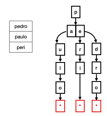
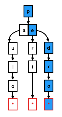
To perform lookups on a trie, you must match each character of the key to the current level of the trie. For example, if you search for pedro, you must check the root contains the letter p. If it does, you check if any of its children contains the letter e, up to the point you reach a leaf node containing the pointer to the tuple that holds this string. (See figure below).
The main advantage of tries is that they have O(k) lookups, meaning that in the worst case, the lookup cost will equal the length of the strings.
In reality, tries can also be used for numeric data types. However, storing them character by character-like strings would be wasteful. Take, for example, the UBIGINT data type. In reality, UBIGINT is a uint64_t which takes 64 bits (i.e., 8 bytes) of space. The maximum value of a uint64_t is 18,446,744,073,709,551,615. Hence if we represented it, like in the example above, we would need 17 levels on the trie. In practice, tries are created on a bit fan-out, which tells how many bits are represented per level of the trie. A uint64_t trie with 8-bit fan-out would have a maximum of 8 levels, each representing a byte.
To have more realistic examples, from this point onwards, all depictions in this post will be with bit representations. In DuckDB, the fan-out is always 8 bits. However, for simplicity, the following examples in this blog post will have a fan-out of 2 bits.
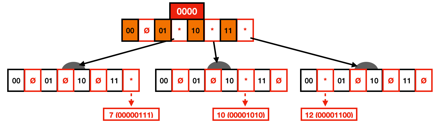
In the example below, we have a trie that indexes the values 7, 10, and 12. You can also see the binary representation of each value on the table next to them. Each node consists of the bits 0 and 1, with a pointer next to them. This pointer can either be set (represented by *) or null (represented by Ø). Similar to the string trie we had before, each level of the trie will represent two bits, with the pointer next to these bits pointing to their children. Finally, the leaves point to the actual data.
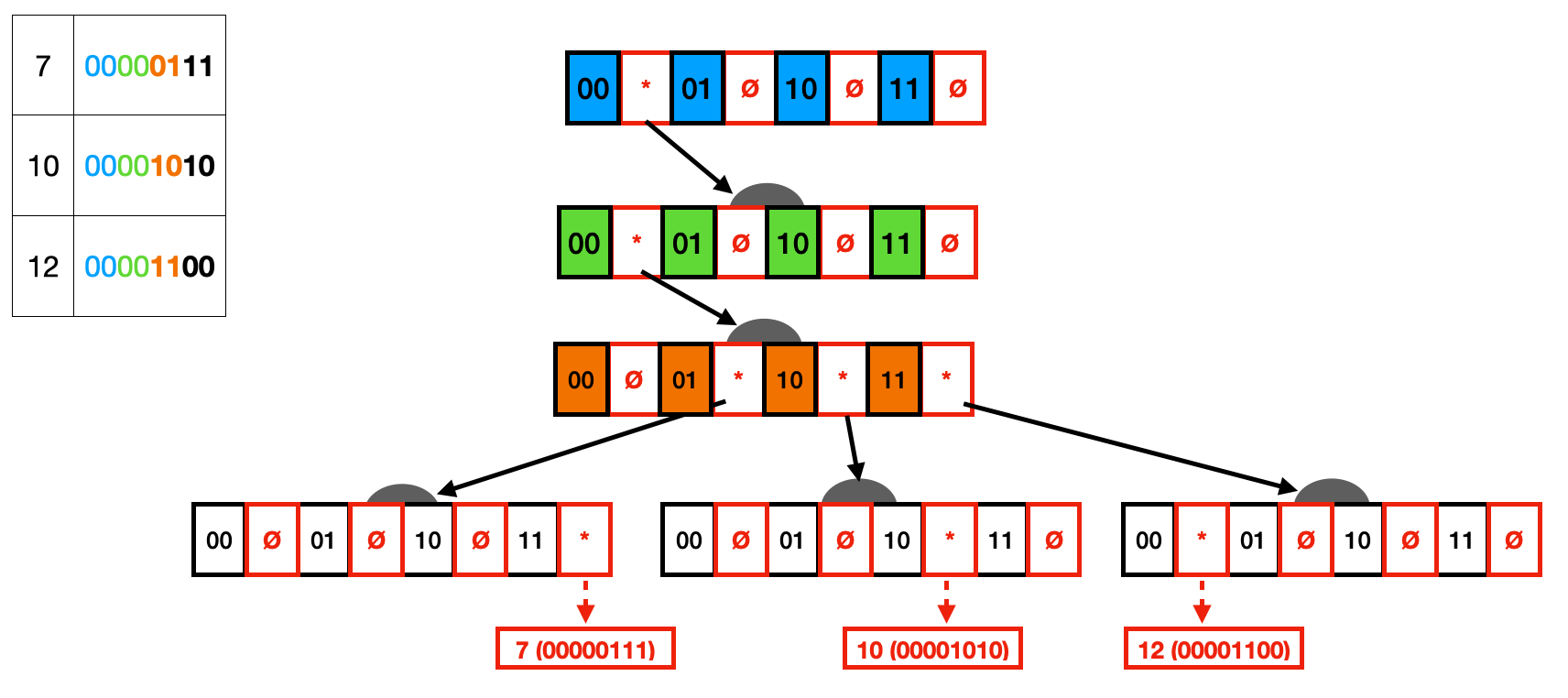
One can quickly notice that this trie representation is wasteful on two different fronts. First, many nodes only have one child (i.e., one path), which could be collapsed by vertical compression (i.e., Radix Tree). Second, many nodes have null pointers, storing space without any information in them, which could be resolved with horizontal compression.
Vertical Compression (i.e., Radix Trees)
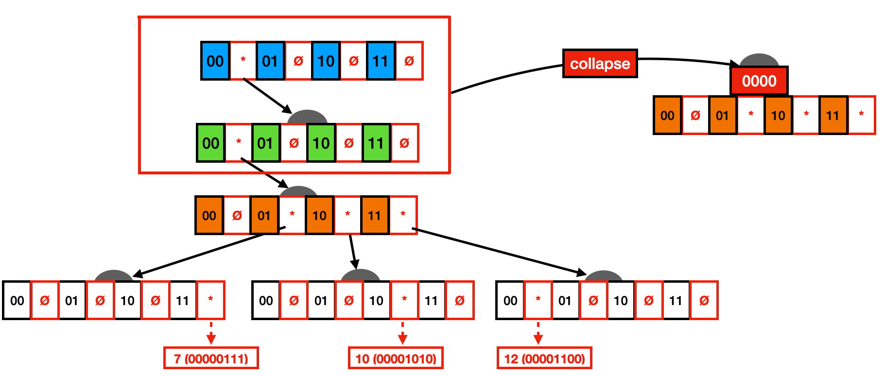
The basic idea of vertical compression is that we collapse paths with nodes that only have one child. To support this, nodes store a prefix variable containing the collapsed path to that node. You can see a representation of this in the figure below. For example, one can see that the first four nodes have only one child. These nodes can be collapsed to the third node (i.e., the first one that bifurcates) as a prefix path. When performing lookups, the key must match all values included in the prefix path.
Below you can see the resulting trie after vertical compression. This trie variant is commonly known as a Radix Tree. Although a lot of wasted space has already been saved with this trie variant, we still have many nodes with unset pointers.
Horizontal Compression (i.e., ART)
To fully understand the design decisions behind ART indexes, we must first extend the 2-bit fan-out to 8-bits, the commonly found fan-out for database systems.
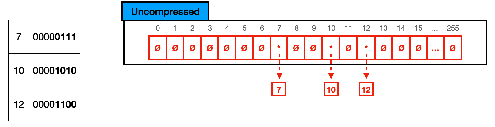
Below you can see the same nodes as before in a trie node of 8 bits. In reality, these nodes will store (2^8) 256 pointers, with the key being the array position of the pointer. In the case depicted by this example, we have a node with (256 pointers * 8 bytes) 2048 byte size while only actually utilizing 24 bytes (3 pointers * 8 bytes), which means that 2016 bytes are entirely wasted. To avoid this situation, ART indexes are composed of 4 different node types that depend on how full the current node is. Below I quickly describe each node with a graphical representation of them. In the graphical representation, I present a conceptual visualization of the node and an example with keys 0,4 and 255.
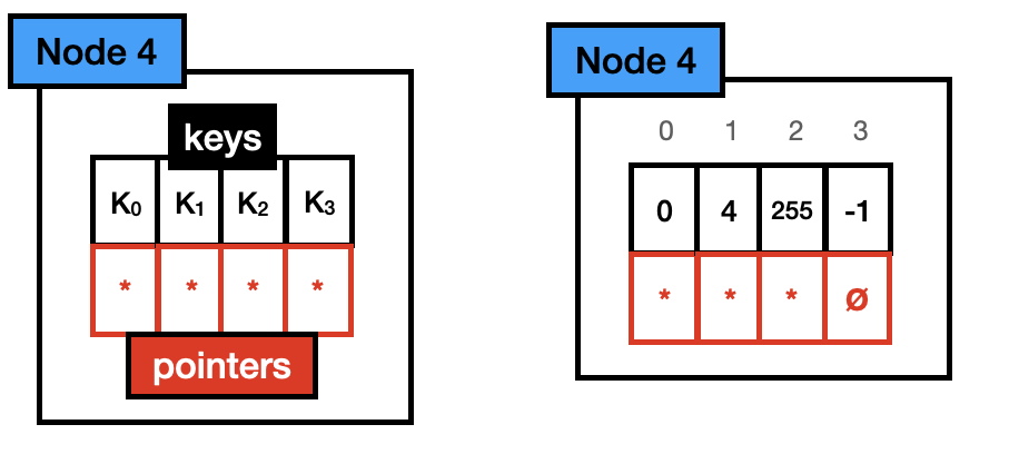
Node 4: Node 4 holds up to 4 different keys. Each key is stored in a one-byte array, with one pointer per key. With its total size being 40 bytes (4*1 + 4*8). Note that the pointer array is aligned with the key array (e.g., key 0 is in position 0 of the keys array, hence its pointer is in position 0 of the pointers array)
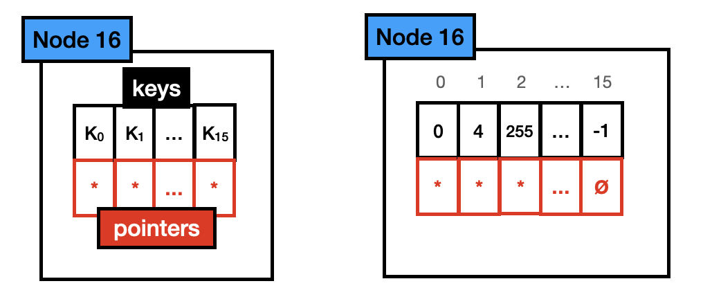
Node 16: Node 16 holds up to 16 different keys. Like node 4, each key is stored in a one-byte array, with one pointer per key. With its total size being 144 bytes (16*1 + 16*8). Like Node 4, the pointer array is aligned with the key array.
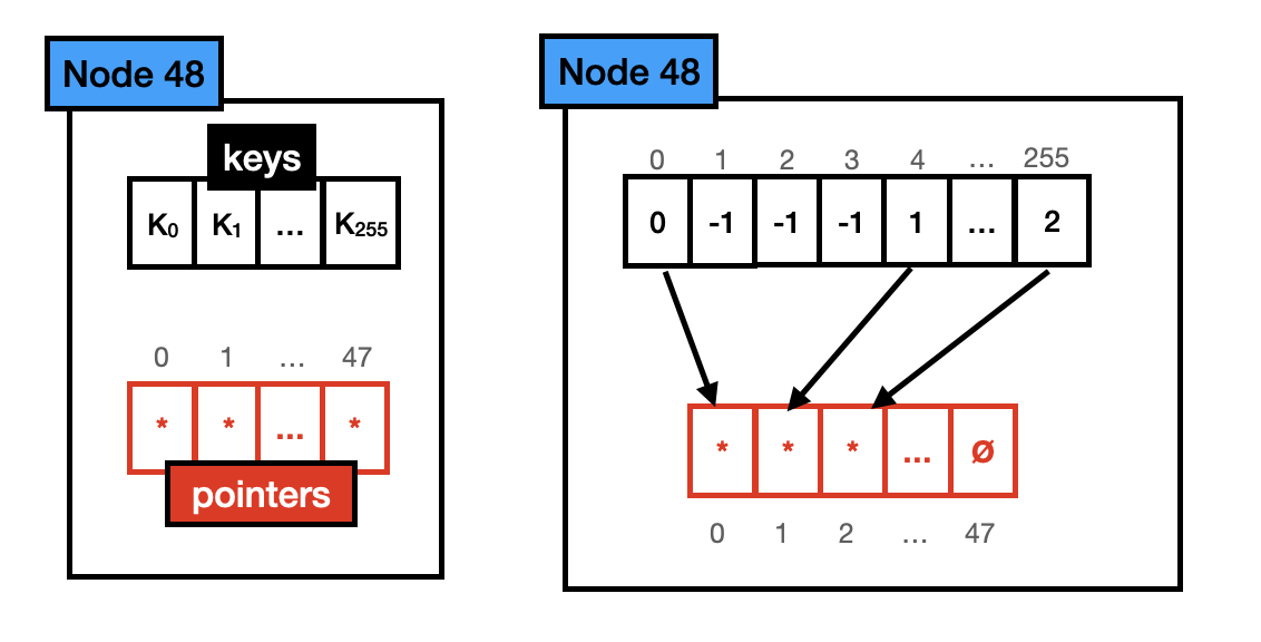
Node 48: Node 48 holds up to 48 different keys. When a key is present in this node, the one-byte array position representing that key will hold an index into the pointer array that points to the child of that key. Its total size is 640 bytes (256*1 + 48*8). Note that the pointer array and the key array are not aligned anymore. The key array points to the position in the pointer array where the pointer of that key is stored (e.g., the key 255 in the key array is set to 2 because the position 2 of the pointer array points to the child pertinent to that key).
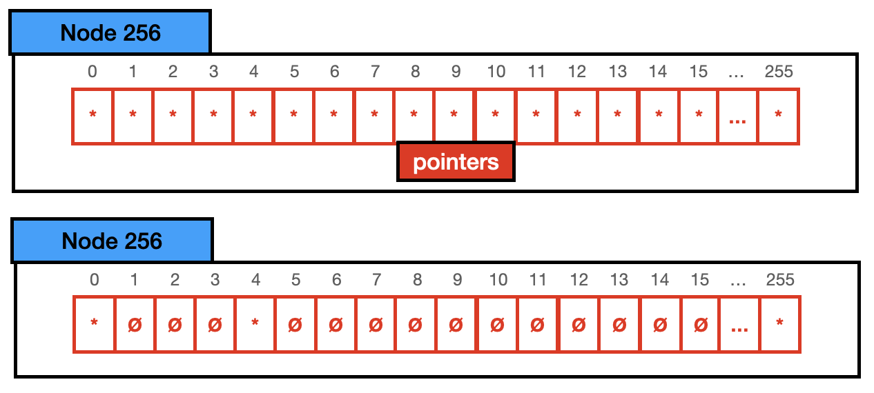
Node 256: Node 256 holds up to 256 different keys, hence all possible values in the distribution. It only has a pointer vector, if the pointer is set, the key exists, and it points to its child. Its total size is 2048 bytes (256 pointers * 8 bytes).
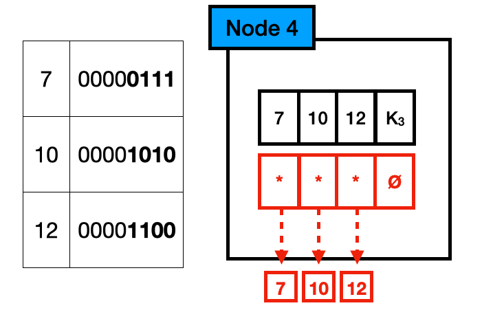
For the example in the previous section, we could use a Node 4 instead of a Node 256 to store the keys, since we only have 3 keys present. Hence it would look like the following:
ART in DuckDB
When considering which index structure to implement in DuckDB, we wanted a structure that could be used to keep PK/FK/Unique constraints while also being able to speed up range queries and Joins. Database systems commonly implement hash tables for constraint checks and B+ trees for range queries. However, we saw in ART Indexes an opportunity to diminish the code complexity by having one data structure for two use cases. The main characteristics that ART Index provides that we take advantage of are:
- Compact structure. Since the ART internal nodes are rather small, they can fit in CPU caches, being a more cache-conscious structure than B+ trees.
- Fast point queries. The worst case for an ART point query is O(k), which is sufficiently fast for constraint checking.
- No dramatic regression on insertions. Many hash table variants must be rebuilt when they reach a certain size. In practice, one insert might cause a significant regression in time, with a query suddenly taking orders of magnitude more time to complete, with no apparent reason for the user. In the ART, inserts might cause node growths (e.g., a Node 4 might grow to a Node 16), but these are inexpensive.
- Ability to run range queries. Although the ART does not run range queries as fast as B+ trees since it must perform tree traversals, where the B+ tree can scan leaf nodes sequentially, it still presents an advantage over hash tables since these types of queries can be done (Some might argue that you can use hash tables for range queries, but meh). This allows us to efficiently use ART for highly selective range queries and index joins.
- Maintainability. Using one structure for both constraint checks and range queries instead of two is more code efficient and maintainable.
What Is It Used For?
As said previously, ART indexes are mainly used in DuckDB on three fronts.
-
Data Constraints. Primary key, Foreign Keys, and Unique constraints are all maintained by an ART Index. When inserting data in a tuple with a constraint, this will effectively try to perform an insertion in the ART index and fail if the tuple already exists.
CREATE TABLE integers (i INTEGER PRIMARY KEY); -- Insert unique values into ART INSERT INTO integers VALUES (3), (2); -- Insert conflicting value in ART will fail INSERT INTO integers VALUES (3); CREATE TABLE fk_integers ( j INTEGER, FOREIGN KEY (j) REFERENCES integers(i) ); -- This insert works normally INSERT INTO fk_integers VALUES (2), (3); -- This fails after checking the ART in integers INSERT INTO fk_integers VALUES (4); -
Range Queries. Highly selective range queries on indexed columns will also use the ART index underneath.
CREATE TABLE integers (i INTEGER PRIMARY KEY); -- Insert unique values into ART INSERT INTO integers VALUES (3), (2), (1), (8) , (10); -- Range queries (if highly selective) will also use the ART index SELECT * FROM integers WHERE i >= 8; -
Joins. Joins with a small number of matches will also utilize existing ART indexes.
-- Optionally you can always force index joins with the following pragma PRAGMA force_index_join; CREATE TABLE t1 (i INTEGER PRIMARY KEY); CREATE TABLE t2 (i INTEGER PRIMARY KEY); -- Insert unique values into ART INSERT INTO t1 VALUES (3), (2), (1), (8), (10); INSERT INTO t2 VALUES (3), (2), (1), (8), (10); -- Joins will also use the ART index SELECT * FROM t1 INNER JOIN t2 ON (t1.i = t2.i); -
Indexes over expressions. ART indexes can also be used to quickly look up expressions.
CREATE TABLE integers (i INTEGER, j INTEGER);

INSERT INTO integers VALUES (1, 1), (2, 2), (3, 3);

-- Creates index over the i + j expression
CREATE INDEX i_index ON integers USING ART((i + j));

-- Uses ART index point query
SELECT i FROM integers WHERE i + j = 2;
ART Storage
There are two main constraints when storing ART indexes:
- The index must be stored in an order that allows for lazy-loading. Otherwise, we would have to fully load the index, including nodes that might be unnecessary to queries that would be executed in that session.
- It must not increase the node size. Otherwise, we diminish the cache-conscious effectiveness of the ART index.
Post-Order Traversal
To allow for lazy loading, we must store all children of a node, collect the information of where each child is stored, and then, when storing the actual node, we store the disk information of each of its children. To perform this type of operation, we do a post-order traversal.
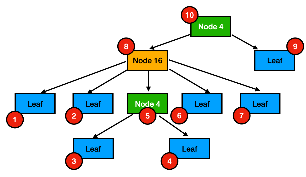
The post-order traversal is shown in the figure below. The circles in red represent the numeric order where the nodes will be stored. If we start from the root node (i.e., Node 4 with storage order 10), we must first store both children (i.e., Node 16 with storage order 8 and the Leaf with storage order 9). This goes on recursively for each of its children.
The figure below shows an actual representation of what this would look like in DuckDB's block format. In DuckDB, data is stored in 256 kB contiguous blocks, with some blocks reserved for metadata and some for actual data. Each block is represented by an id. To allow for navigation within a block, they are partitioned by byte offsets hence each block contains 256,000 different offsets
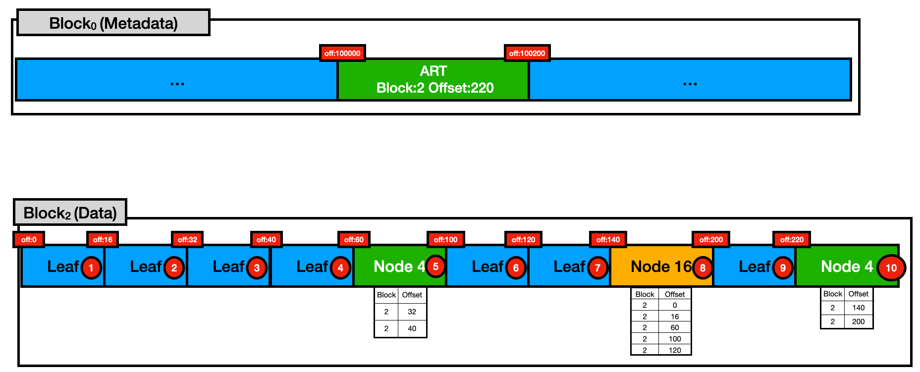
In this example, we have Block 0 that stored some of our database metadata. In particular, between offsets 100,000 and 100,200 we store information pertinent to one ART index. This will store information on the index (e.g., name, constraints, expression) and the <Block,Offset> position of its root node.
For example, let's assume we are doing a lookup of the key with row_ids stored in the Leaf with storage order 1. We would start by loading the Art Root node on <Block:2, Offset:220>, by checking the keys stored in that Node, we would then see we must load the Node 16 at <Block:2, Offset:140>, and then finally our Leaf at <Block:0, Offset:0>. That means that for this lookup, only these 3 nodes were loaded into memory. Subsequent access to these nodes would only require memory access, while access to different nodes (e.g., Leaf storage order 2) would still result in disk access.
One major problem with implementing this (de)serialization process is that now we not only have to keep information about the memory address of pointers but also if they are already in memory and if not, what's the <Block,Offset> position they are stored.
If we stored the Block Id and Offset in new variables, it would dramatically increase the ART node sizes, diminishing its effectiveness as a cache-conscious data structure.
Take Node 256 as an example. The cost of holding 256 pointers is 2048 bytes (256 pointers * 8 bytes). Let's say we decide to store the Block Information on a new array like the following:
struct BlockPointer {
    uint32_t block_id;
    uint32_t offset;
}

class Node256 : public Node  {
    // Pointers to the child nodes
    Node* children[256];
    BlockPointer block_info[256];
}
Node 256 would increase 2048 bytes (256 * (4+4)), causing it to double its current size to 4096 bytes.
Pointer Swizzling
To avoid the increase in sizes of ART nodes, we decided to implement Swizzlable Pointers and use them instead of regular pointers.
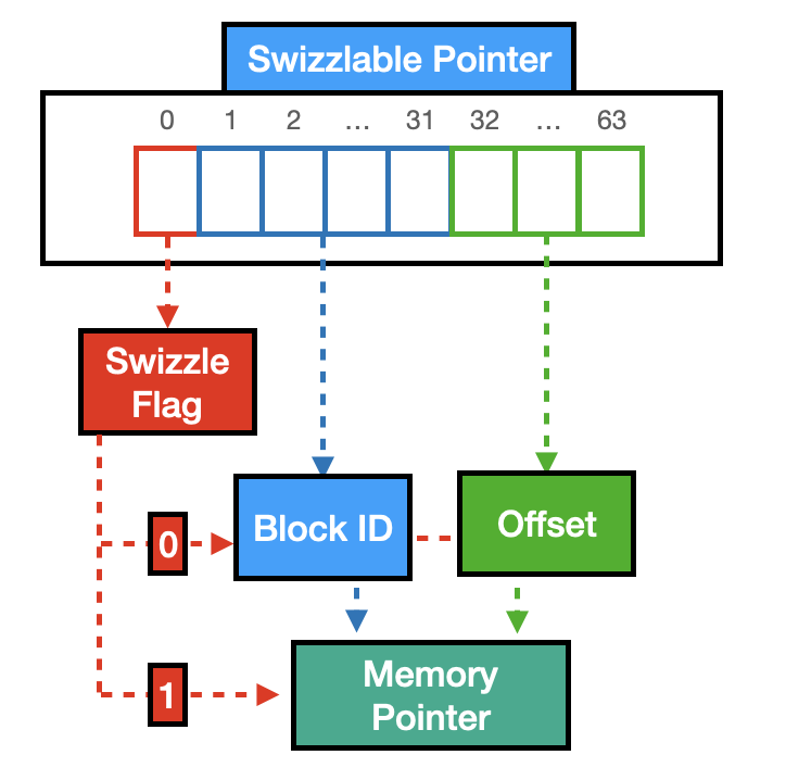
The idea is that we don't need all 64 bits (i.e., 48 bits give you an address space of 256 terabytes, supporting any of the current architectures, see the related discussion on Stack Overflow and the “64-bit computing” Wikipedia page) in a pointer to point to a memory address. Hence we can use the most significant bit as a flag (i.e., the Swizzle Flag). If the swizzle flag is set, the value in our Swizzlable Pointer is a memory address for the Node. Otherwise, the variable stores the Block Information of where the Node is stored. In the latter case, we use the following 31 bits to store the Block ID and the remaining 32 bits to store the offset.
In the following figure, you can see a visual representation of DuckDB's Swizzlable Pointer.
Benchmarks
To evaluate the benefits and disadvantages of our current storage implementation, we run a benchmark (Available at this Colab Link), where we create a table containing 50,000,000 integral elements with a primary key constraint on top of them.
con = duckdb.connect("vault.db")
con.execute("CREATE TABLE integers (x INTEGER PRIMARY KEY)")
con.execute("INSERT INTO integers SELECT * FROM range(50000000)")
We run this benchmark on two different versions of DuckDB, one where the index is not stored (i.e., v0.4.0), which means it is always in memory and fully reconstructed at a database restart, and another one where the index is stored (i.e., bleeding-edge version), using the lazy-loading technique described previously.
Storing Time
We first measure the additional cost of serializing our index.
cur_time = time.time()
con.close()
print("Storage time: " + str(time.time() - cur_time))
Storage Time
| Name | Time (s) |
|---|---|
| Reconstruction | 8.99 |
| Storage | 18.97 |
We can see storing the index is 2x more expensive than not storing the index. The reason is that our table consists of one column with 50,000,000 int32_t values. However, when storing the ART, we also store 50,000,000 int64_t values for their respective row_ids in the leaves. This increase in the elements is the main reason for the additional storage cost.
Load Time
We now measure the loading time of restarting our database.
cur_time = time.time()
con = duckdb.connect("vault.db")
print("Load time: " + str(time.time() - cur_time))
| Name | Time (s) |
|---|---|
| Reconstruction | 7.75 |
| Storage | 0.06 |
Here we can see a two-order magnitude difference in the times of loading the database. This difference is basically due to the complete reconstruction of the ART index during loading. In contrast, in the Storage version, only the metadata information about the ART index is loaded at this point.
Query Time (Cold)
We now measure the cold query time (i.e., the Database has just been restarted, which means that in the Storage version, the index does not exist in memory yet.) of running point queries on our index. We run 5000 point queries, equally spaced on 10000 elements in our distribution. We use this value to always force the point queries to load a large number of unused nodes.
times = []
for i in range (0, 50000000, 10000):
  cur_time = time.time()
  con.execute("SELECT x FROM integers WHERE x = " + str(i))
  times.append(time.time() - cur_time)
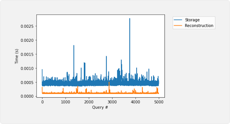
In general, each query is 3x more expensive in the persisted storage format. This is due to two main reasons:
- Creating the nodes. In the storage version, we do create the nodes lazily, which means that, for each node, all parameters must be allocated, and values like keys and prefixes are loaded.
- Block pinning. At every node, we must pin and unpin the blocks where they are stored.
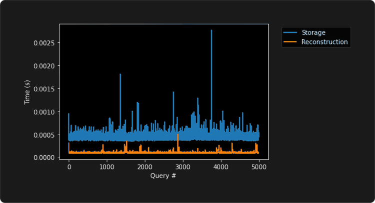
Query Time (Hot)
In this experiment, we execute the same queries as in the previous section.
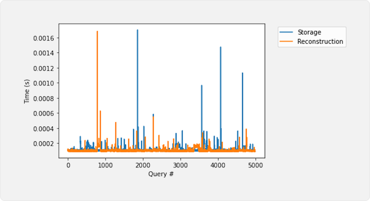
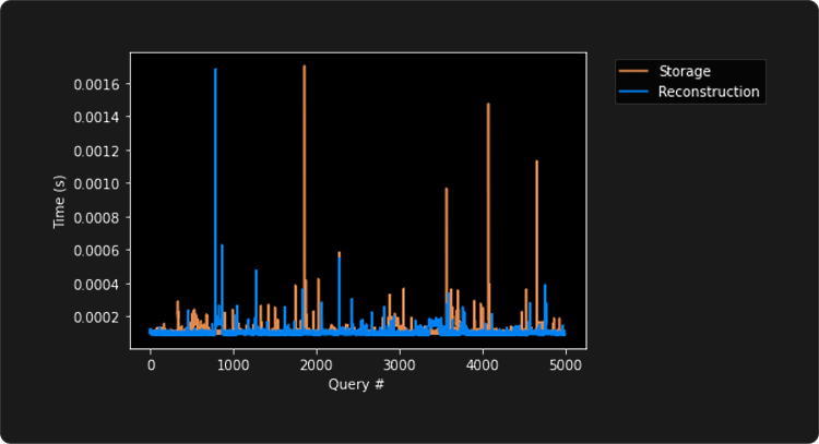
The times in both versions are comparable since all the nodes in the storage version are already set in memory. In conclusion, when stored indexes are in active use, they present similar performance to fully in-memory indexes.
Future Work
ART index storage has been a long-standing issue in DuckDB, with multiple users claiming it was a missing feature that created an impediment for them to use DuckDB. Although now storing and lazily loading ART indexes is possible, there are many future paths we can still pursue to make the ART-Index more performant. Here I list what I believe are the most important next steps:
- Caching pinned blocks. In our current implementation, blocks are constantly pinned and unpinned, even though blocks can store multiple nodes and are most likely reused continuously through lookups. Smartly caching them will result in drastic savings for queries that trigger node loading.
- Bulk loading. Our ART-Index currently does not support bulk loading. This means that nodes will be constantly resized when creating an index over a column since elements will be inserted one by one. If we bulk-load the data, we can know exactly which Nodes we must create for that dataset, hence avoiding these frequent resizes.
- Bulk insertion. When performing bulk insertion, a similar problem as bulk-loading would happen. A possible solution would be to create a new ART index with Bulk-Loading and then merge it with the existing ART index.
- Vectorized lookups/inserts. DuckDB utilized a vectorized execution engine. However, both our ART lookups and inserts still follow a tuple-at-a-time model.
- Updatable index storage. In our current implementation, ART-Indexes are fully invalidated from disk and stored again. This causes an unnecessary increase in storage time on subsequent storage. Updating nodes directly into disk instead of entirely rewriting the index could drastically decrease future storage costs. In other words, indexes are constantly completely stored at every checkpoint.
- Combined pointer/row id leaves. Our current leaf node format allows for storing values that are repeated over multiple tuples. However, since ART indexes are commonly used to keep unique key constraints (e.g., Primary Keys), and a unique
row_idfits in the same pointer size space, a lot of space can be saved by using the child pointers to point to the actualrow_idinstead of creating an actual leaf node that only stores onerow_id.
Roadmap
It's tough to make predictions, especially about the future
– Yogi Berra
ART Indexes are a core part of both constraint enforcement and keeping access speed up in DuckDB. And as depicted in the previous section, there are many distinct paths we can take in our bag of ART goodies, with advantages for completely different use cases.