Linearization/Delinearization, Z-Order, Hilbert and Morton Curves
Installing and Loading
INSTALL lindel FROM community;
LOAD lindel;
Example
WITH elements AS (
  SELECT * AS id FROM range(3)
)
SELECT
  a.id AS a,
  b.id AS b,
  hilbert_encode([a.id, b.id]::tinyint[2]) AS hilbert,
  morton_encode([a.id, b.id]::tinyint[2]) AS morton
FROM
  elements AS a CROSS JOIN elements AS b;
┌───────┬───────┬─────────┬────────┐
│   a   │   b   │ hilbert │ morton │
│ int64 │ int64 │ uint16  │ uint16 │
├───────┼───────┼─────────┼────────┤
│     0 │     0 │       0 │      0 │
│     0 │     1 │       3 │      1 │
│     0 │     2 │       4 │      4 │
│     1 │     0 │       1 │      2 │
│     1 │     1 │       2 │      3 │
│     1 │     2 │       7 │      6 │
│     2 │     0 │      14 │      8 │
│     2 │     1 │      13 │      9 │
│     2 │     2 │       8 │     12 │
└───────┴───────┴─────────┴────────┘

-- Encode two 32-bit floats into one uint64
SELECT hilbert_encode([37.8, .2]::float[2]) AS hilbert;
┌─────────────────────┐
│       hilbert       │
│       uint64        │
├─────────────────────┤
│ 2303654869236839926 │
└─────────────────────┘

-- Since doubles use 64 bits of precision the encoding
-- must result in a uint128

SELECT hilbert_encode([37.8, .2]::double[2]) AS hilbert;
┌────────────────────────────────────────┐
│                hilbert                 │
│                uint128                 │
├────────────────────────────────────────┤
│ 42534209309512799991913666633619307890 │
└────────────────────────────────────────┘

-- 3 dimensional encoding.
SELECT hilbert_encode([1.0, 5.0, 6.0]::float[3]) AS hilbert;
┌──────────────────────────────┐
│           hilbert            │
│           uint128            │
├──────────────────────────────┤
│ 8002395622101954260073409974 │
└──────────────────────────────┘

-- Demonstrate string encoding
SELECT hilbert_encode([ord(x) for x in split('abcd', '')]::tinyint[4]) AS hilbert;
┌───────────┐
│  hilbert  │
│  uint32   │
├───────────┤
│ 178258816 │
└───────────┘

-- Start out just by encoding two values.
SELECT hilbert_encode([1, 2]::tinyint[2]) AS hilbert;
┌─────────┐
│ hilbert │
│ uint16  │
├─────────┤
│       7 │
└─────────┘

-- Decode an encoded value
SELECT hilbert_decode(7::uint16, 2, false, true) AS values;
┌─────────────┐
│   values    │
│ utinyint[2] │
├─────────────┤
│ [1, 2]      │
└─────────────┘

-- The decoding functions take four parameters:
-- 1. **Value to be decoded:** This is always an unsigned integer type.
-- 2. **Number of elements to decode:** This is a `TINYINT` specifying how many elements should be decoded.
-- 3. **Float return type:** This `BOOLEAN` indicates whether the values should be returned as floats (REAL or DOUBLE). Set to true to enable this.
-- 4. **Unsigned return type:** This `BOOLEAN` indicates whether the values should be unsigned if not using floats.
-- The return type of these functions is always an array, with the element type determined by the number of elements requested and whether "float" handling is enabled by the third parameter.

SELECT hilbert_decode(hilbert_encode([1, -2]::bigint[2]), 2, false, false) AS values;
┌───────────┐
│  values   │
│ bigint[2] │
├───────────┤
│ [1, -2]   │
└───────────┘
About lindel
This lindel extension adds functions for the linearization and
delinearization of numeric arrays in DuckDB. It allows you to order
multi-dimensional data using space-filling curves.
What is linearization?
Linearization maps multi-dimensional data into a one-dimensional sequence while preserving locality, enhancing the efficiency of data structures and algorithms for spatial data, such as in databases, GIS, and memory caches.
"The principle of locality states that programs tend to reuse data and instructions they have used recently."
In SQL, sorting by a single column (e.g., time or identifier) is often sufficient, but sometimes queries involve multiple fields, such as:
- Time and identifier (historical trading data)
- Latitude and Longitude (GIS applications)
- Latitude, Longitude, and Altitude (flight tracking)
- Latitude, Longitude, Altitude, and Time (flight history)
Sorting by a single field isn't optimal for multi-field queries. Linearization maps multiple fields into a single value, while preserving locality—meaning values close in the original representation remain close in the mapped representation.
Where has this been used before?
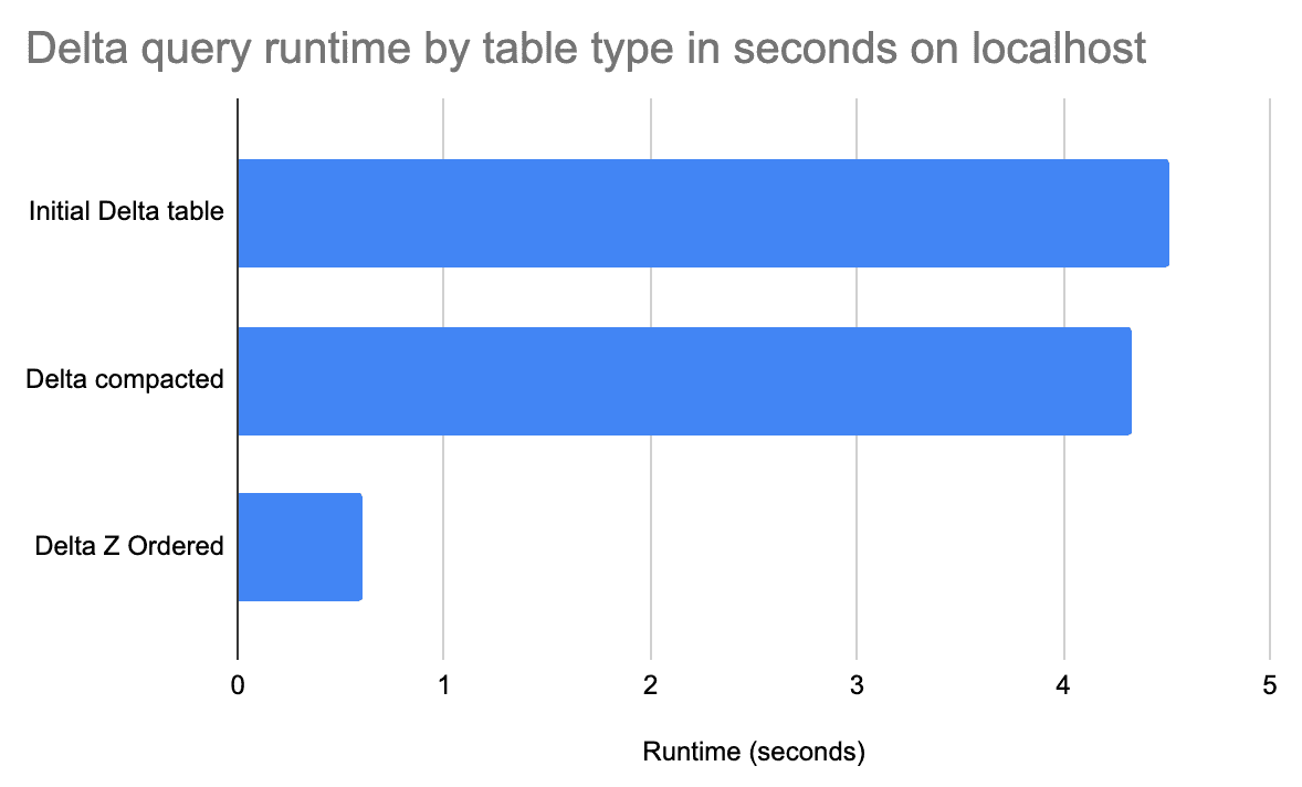
DataBricks has long supported Z-Ordering (they also now default to using the Hilbert curve for the ordering). This video explains how Delta Lake queries are faster when the data is Z-Ordered. This extension also allows DuckDB to write files with the same ordering optimization.
Numerous articles describe the benefits of applying a Z-Ordering/Hilbert ordering to data for query performance.
- https://delta.io/blog/2023-06-03-delta-lake-z-order/
- https://blog.cloudera.com/speeding-up-queries-with-z-order/
- https://www.linkedin.com/pulse/z-order-visualization-implementation-nick-karpov/
From one of the articles:

Your particular performance improvements will vary, but for some query patterns Z-Ordering and Hilbert ordering will make quite a big difference.
When would I use this?
For query patterns across multiple numeric or short text columns, consider sorting rows using Hilbert encoding when storing data in Parquet:
COPY (
  SELECT * FROM 'source.csv'
  order by
  hilbert_encode([source_data.time, source_data.symbol_id]::integer[2])
)
TO 'example.parquet' (FORMAT PARQUET)

-- or if dealing with latitude and longitude

COPY (
  SELECT * FROM 'source.csv'
  order by
  hilbert_encode([source_data.lat, source_data.lon]::double[2])
) TO 'example.parquet' (FORMAT PARQUET)
The Parquet file format stores statistics for each row group. Since rows are sorted with locality into these row groups the query execution may be able to skip row groups that contain no relevant rows, leading to faster query execution times.
Encoding Types
This extension offers two different encoding types, Hilbert and Morton encoding.
Hilbert Encoding
Hilbert encoding uses the Hilbert curve, a continuous fractal space-filling curve named after David Hilbert. It rearranges coordinates based on the Hilbert curve's path, preserving spatial locality better than Morton encoding.
This is a great explanation of the Hilbert curve.
Morton Encoding (Z-order Curve)
Morton encoding, also known as the Z-order curve, interleaves the binary representations of coordinates into a single integer. It is named after Glenn K. Morton.
Locality: Hilbert encoding generally preserves locality better than Morton encoding, making it preferable for applications where spatial proximity matters.
Encoded Output is limited to a 128-bit UHUGEINT. The input array size is validated to ensure it fits within this limit.
| Input Type | Maximum Number of Elements | Output Type (depends on number of elements) |
|---|---|---|
UTINYINT |
16 | 1: UTINYINT2: USMALLINT3-4: UINTEGER4-8: UBIGINT8-16: UHUGEINT |
USMALLINT |
8 | 1: USMALLINT2: UINTEGER3-4: UBIGINT4-8: UHUGEINT |
UINTEGER |
4 | 1: UINTEGER2: UBIGINT3-4: UHUGEINT |
UBIGINT |
2 | 1: UBIGINT2: UHUGEINT |
FLOAT |
4 | 1: UINTEGER2: UBIGINT3-4: UHUGEINT |
DOUBLE |
2 | 1: UBIGINT2: UHUGEINT |
Added Functions
| function_name | function_type | description | comment | examples |
|---|---|---|---|---|
| hilbert_encode | scalar | Encode an array of values using the Hilbert space filling curve | NULL | [select hilbert_encode([43, 3]::integer[2]);] |
| hilbert_decode | scalar | Decode a Hilbert encoded set of values | NULL | [select hilbert_decode(7::uint16, 2, false, true) as values;] |
| morton_encode | scalar | Encode an array of values using Morton encoding | NULL | [select morton_encode([43, 3]::integer[2]);] |
| morton_decode | scalar | Decode an array of values using Morton encoding | NULL | [select morton_decode(7::uint16, 2, false, true) as values;] |
