Windowing in DuckDB
TL;DR: DuckDB, a free and open-source analytical data management system, has a state-of-the-art windowing engine that can compute complex moving aggregates like inter-quartile ranges as well as simpler moving averages.
Window functions (those using the OVER clause) are important tools for analyzing data series,
but they can be slow if not implemented carefully.
In this post, we will take a look at how DuckDB implements windowing.
We will also see how DuckDB can leverage its aggregate function architecture
to compute useful moving aggregates such as moving inter-quartile ranges (IQRs).
Beyond Sets
The original relational model as developed by Codd in the 1970s treated relations as unordered sets of tuples.
While this was nice for theoretical computer science work,
it ignored the way humans think using physical analogies (the "embodied brain" model from neuroscience).
In particular, humans naturally order data to help them understand it and engage with it.
To help with this, SQL uses the SELECT clause for horizontal layout and the ORDER BY clause for vertical layout.
Still, the orderings that humans put on data are often more than neurological crutches. For example, time places a natural ordering on measurements, and wide swings in those measurements can themselves be important data, or they may indicate that the data needs to be cleaned by smoothing. Trends may be present or relative changes may be more important for analysis than raw values. To help answer such questions, SQL introduced analytic (or window) functions in 2003.
Window Functions
Windowing works by breaking a relation up into independent partitions, ordering those partitions,
and then defining various functions that can be computed for each row
using the nearby values.
These functions include all the aggregate functions (such as sum and avg)
as well as some window-specific functions (such as rank() and nth_value(<expression>, <N>)).
Some window functions depend only on the partition boundary and the ordering, but a few (including all the aggregates) also use a frame. Frames are specified as a number of rows on either side (preceding or following) of the current row. The distance can either be specified as a number of rows or a range of values using the partition's ordering value and a distance.
Framing is the most confusing part of the windowing environment, so let's look at a very simple example and ignore the partitioning and ordering for a moment.
SELECT points,
    sum(points) OVER (
        ROWS BETWEEN 1 PRECEDING
                 AND 1 FOLLOWING) AS we
FROM results;
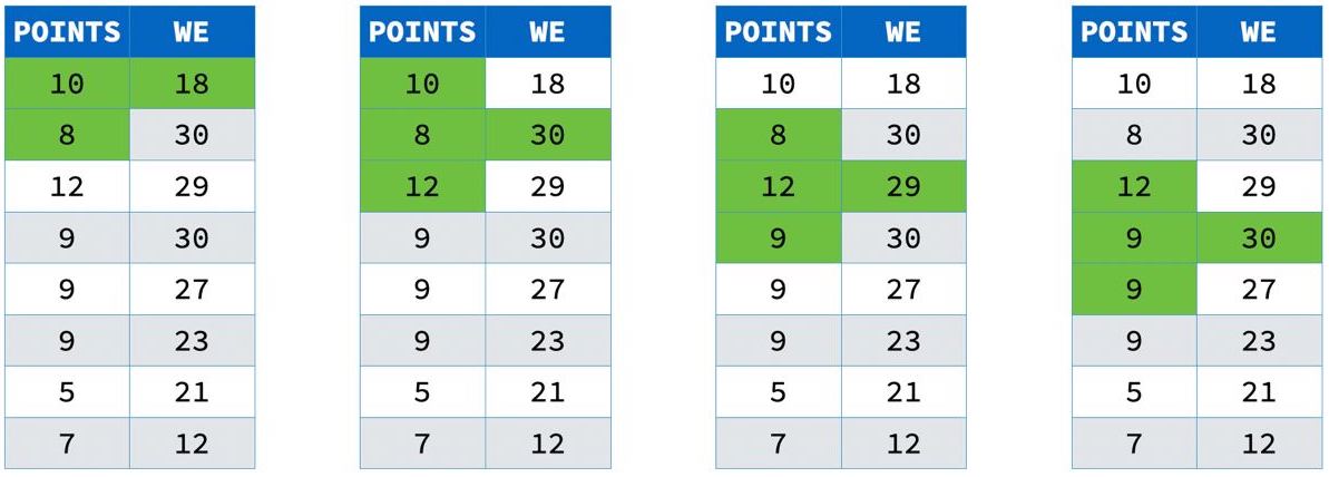
This query computes the sum of each point and the points on either side of it:

Notice that at the edge of the partition, there are only two values added together.
Power Generation Example
Now let's look at a concrete example of a window function query. Suppose we have some power plant generation data:
| Plant | Date | MWh |
|---|---|---|
| Boston | 2019-01-02 | 564337 |
| Boston | 2019-01-03 | 507405 |
| Boston | 2019-01-04 | 528523 |
| Boston | 2019-01-05 | 469538 |
| Boston | 2019-01-06 | 474163 |
| Boston | 2019-01-07 | 507213 |
| Boston | 2019-01-08 | 613040 |
| Boston | 2019-01-09 | 582588 |
| Boston | 2019-01-10 | 499506 |
| Boston | 2019-01-11 | 482014 |
| Boston | 2019-01-12 | 486134 |
| Boston | 2019-01-13 | 531518 |
| Worcester | 2019-01-02 | 118860 |
| Worcester | 2019-01-03 | 101977 |
| Worcester | 2019-01-04 | 106054 |
| Worcester | 2019-01-05 | 92182 |
| Worcester | 2019-01-06 | 94492 |
| Worcester | 2019-01-07 | 99932 |
| Worcester | 2019-01-08 | 118854 |
| Worcester | 2019-01-09 | 113506 |
| Worcester | 2019-01-10 | 96644 |
| Worcester | 2019-01-11 | 93806 |
| Worcester | 2019-01-12 | 98963 |
| Worcester | 2019-01-13 | 107170 |
The data is noisy, so we want to compute a 7 day moving average for each plant. To do this, we can use this window query:
SELECT "Plant", "Date",
    avg("MWh") OVER (
        PARTITION BY "Plant"
        ORDER BY "Date" ASC
        RANGE BETWEEN INTERVAL 3 DAYS PRECEDING
                  AND INTERVAL 3 DAYS FOLLOWING)
        AS "MWh 7-day Moving Average"
FROM "Generation History"
ORDER BY 1, 2;
This query computes the seven day moving average of the power generated by each power plant on each day.
The OVER clause is the way that SQL specifies that a function is to be computed in a window.
It partitions the data by Plant (to keep the different power plants' data separate),
orders each plant's partition by Date (to put the energy measurements next to each other),
and uses a RANGE frame of three days on either side of each day for the avg
(to handle any missing days).
Here is the result:
| Plant | Date | MWh 7-day Moving Average |
|---|---|---|
| Boston | 2019-01-02 | 517450.75 |
| Boston | 2019-01-03 | 508793.20 |
| Boston | 2019-01-04 | 508529.83 |
| Boston | 2019-01-05 | 523459.85 |
| Boston | 2019-01-06 | 526067.14 |
| Boston | 2019-01-07 | 524938.71 |
| Boston | 2019-01-08 | 518294.57 |
| Boston | 2019-01-09 | 520665.42 |
| Boston | 2019-01-10 | 528859.00 |
| Boston | 2019-01-11 | 532466.66 |
| Boston | 2019-01-12 | 516352.00 |
| Boston | 2019-01-13 | 499793.00 |
| Worcester | 2019-01-02 | 104768.25 |
| Worcester | 2019-01-03 | 102713.00 |
| Worcester | 2019-01-04 | 102249.50 |
| Worcester | 2019-01-05 | 104621.57 |
| Worcester | 2019-01-06 | 103856.71 |
| Worcester | 2019-01-07 | 103094.85 |
| Worcester | 2019-01-08 | 101345.14 |
| Worcester | 2019-01-09 | 102313.85 |
| Worcester | 2019-01-10 | 104125.00 |
| Worcester | 2019-01-11 | 104823.83 |
| Worcester | 2019-01-12 | 102017.80 |
| Worcester | 2019-01-13 | 99145.75 |
You can request multiple different OVER clauses in the same SELECT, and each will be computed separately.
Often, however, you want to use the same window for multiple functions,
and you can do this by using a WINDOW clause to define a named window:
SELECT "Plant", "Date",
    avg("MWh") OVER seven AS "MWh 7-day Moving Average"
FROM "Generation History"
WINDOW seven AS (
    PARTITION BY "Plant"
    ORDER BY "Date" ASC
    RANGE BETWEEN INTERVAL 3 DAYS PRECEDING
              AND INTERVAL 3 DAYS FOLLOWING)
ORDER BY 1, 2;
This would be useful, for example,
if one also wanted the 7-day moving min and max to show the bounds of the data.
Under the Feathers
That is a long list of complicated functionality! Making it all work relatively quickly has many pieces, so lets have a look at how they all get implemented in DuckDB.
Pipeline Breaking
The first thing to notice is that windowing is a "pipeline breaker".
That is, the Window operator has to read all of its inputs before it can start computing a function.
This means that if there is some other way to compute something,
it may well be faster to use a different technique.
One common analytic task is to find the last value in some group.
For example, suppose we want the last recorded power output for each plant.
It is tempting to use the rank() window function with a reverse sort for this task:
SELECT "Plant", "MWh"
FROM (
    SELECT "Plant", "MWh",
        rank() OVER (
            PARTITION BY "Plant"
            ORDER BY "Date" DESC) AS r
    FROM table) t
WHERE r = 1;
but this requires materialising the entire table, partitioning it, sorting the partitions,
and then pulling out a single row from those partitions.
A much faster way to do this is to use a self join to filter the table
to contain only the last (max) value of the DATE field:
SELECT table."Plant", "MWh"
FROM table,
    (SELECT "Plant", max("Date") AS "Date"
     FROM table GROUP BY 1) lasts
WHERE table."Plant" = lasts."Plant"
  AND table."Date" = lasts."Date";
This join query requires two scans of the table, but the only materialised data is the filtering table (which is probably much smaller than the original table), and there is no sorting at all.
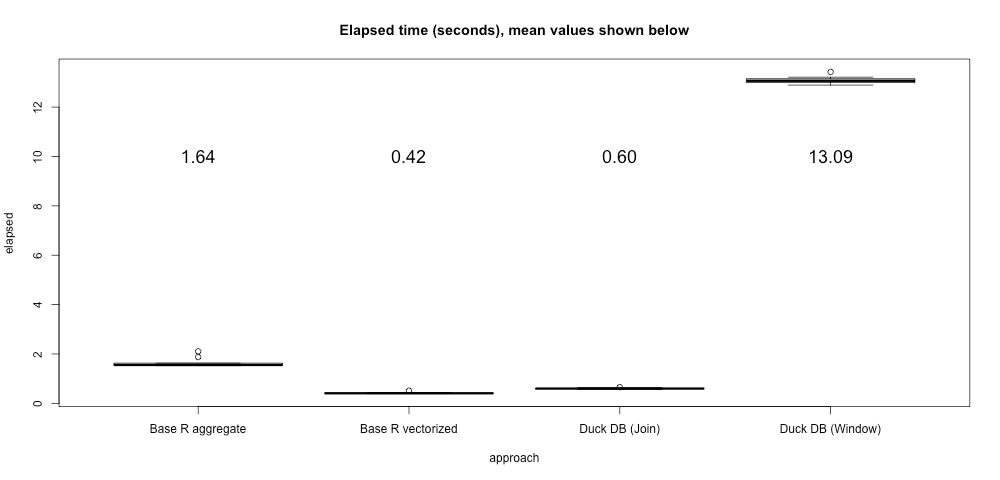
This type of query showed up in a user's blog and we found that the join query was over 20 times faster on their data set:

Of course most analytic tasks that use windowing do require using the Window operator,
and DuckDB uses a collection of techniques to make the performance as fast as possible.
Partitioning and Sorting
At one time, windowing was implemented by sorting on both the partition and the ordering fields
and then finding the partition boundaries.
This is resource intensive, both because the entire relation must be sorted,
and because sorting is O(N log N) in the size of the relation.
Fortunately, there are faster ways to implement this step.
To reduce resource consumption, DuckDB uses the partitioning scheme from Leis et al.'s
Efficient Processing of Window Functions in Analytical SQL Queries
and breaks the partitions up into 1024 chunks using O(N) hashing.
The chunks still need to be sorted on all the fields because there may be hash collisions,
but each partition can now be 1024 times smaller, which reduces the runtime significantly.
Moreover, the partitions can easily be extracted and processed in parallel.
Sorting in DuckDB recently got a big performance boost,
along with the ability to work on partitions that were larger than memory.
This functionality has been also added to the Window operator,
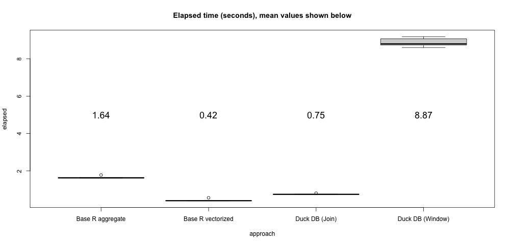
resulting in a 33% improvement in the last-in-group example:

As a final optimization, even though you can request multiple window functions, DuckDB will collect functions that use the same partitioning and ordering, and share the data layout between those functions.
Aggregation
Most of the general-purpose window functions are straightforward to compute, but windowed aggregate functions can be expensive because they need to look at multiple values for each row. They often need to look at the same value multiple times, or repeatedly look at a large number of values, so over the years several approaches have been taken to improve performance.
Naïve Windowed Aggregation
Before explaining how DuckDB implements windowed aggregation, we need to take a short detour through how ordinary aggregates are implemented. Aggregate "functions" are implemented using three required operations and one optional operation:
- Initialize – Creates a state that will be updated.
For
sum, this is the running total, starting atNULL(because asumof zero items isNULL, not zero.) - Update – Updates the state with a new value. For
sum, this adds the value to the state. - Finalize – Produces the final aggregate value from the state.
For
sum, this just copies the running total. - Combine – Combines two states into a single state.
Combine is optional, but when present it allows the aggregate to be computed in parallel.
For
sum, this produces a new state with the sum of the two input values.
The simplest way to compute an individual windowed aggregate value is to initialize a state,
update the state with all the values in the window frame,
and then use finalize to produce the value of the windowed aggregate.
This naïve algorithm will always work, but it is quite inefficient.
For example, a running total will re-add all the values from the start of the partition
for each running total, and this has a run time of O(N^2).
To improve on this, some databases add additional
"moving state" operations
that can add or remove individual values incrementally.
This reduces computation in some common cases,
but it can only be used for certain aggregates.
For example, it doesn't work for min) because you don't know if there are multiple duplicate minima.
Moreover, if the frame boundaries move around a lot, it can still degenerate to an O(N^2) run time.
Segment Tree Aggregation
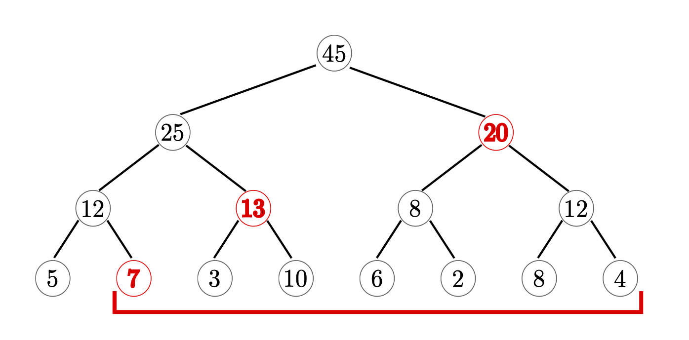
Instead of adding more functions, DuckDB uses the segment tree approach from Leis et al. above. This works by building a tree on top of the entire partition with the aggregated values at the bottom. Values are combined into states at nodes above them in the tree until there is a single root:

To compute a value, the algorithm generates states for the ragged ends of the frame, combines states in the tree above the values in the frame, and finalizes the result from the last remaining state. So in the example above (Figure 5 from Leis et al.) only three values need to be added instead of 7. This technique can be used for all combinable aggregates.
General Windowed Aggregation
The biggest drawback of segment trees is the need to manage a potentially large number of intermediate states.
For the simple states used for standard distributive aggregates like sum,
this is not a problem because the states are small,
the tree keeps the number of states logarithmically low,
and the state used to compute each value is also cheap.
For some aggregates, however, the state is not small.
Typically these are so-called holistic aggregates,
where the value depends on all the values of the frame.
Examples of such aggregates are mode and quantile,
where each state may have to contain a copy of all the values seen so far.
While segment trees can be used to implement moving versions of any combinable aggregate,
this can be quite expensive for large, complex states –
and this was not the original goal of the algorithm.
To solve this problem, we use the approach from Wesley and Xu's Incremental Computation of Common Windowed Holistic Aggregates, which generalises segment trees to aggregate-specific data structures. The aggregate can define a fifth optional window operation, which will be passed the bottom of the tree and the bounds of the current and previous frame. The aggregate can then create an appropriate data structure for its implementation.
For example, the mode function maintains a hash table of counts that it can update efficiently,
and the quantile function maintains a partially sorted list of frame indexes.
Moreover, the quantile functions can take an array of quantile values,
which further increases performance by sharing the partially ordered results
among the different quantile values.
Because these aggregates can be used in a windowing context, the moving average example above can be easily modified to produce a moving inter-quartile range:
SELECT "Plant", "Date",
    quantile_cont("MWh", [0.25, 0.5, 0.75]) OVER seven
        AS "MWh 7-day Moving IQR"
FROM "Generation History"
WINDOW seven AS (
    PARTITION BY "Plant"
    ORDER BY "Date" ASC
    RANGE BETWEEN INTERVAL 3 DAYS PRECEDING
              AND INTERVAL 3 DAYS FOLLOWING)
ORDER BY 1, 2;
Moving quantiles like this are more robust to anomalies, which makes them a valuable tool for data series analysis, but they are not generally implemented in most database systems. There are some approaches that can be used in some query engines, but the lack of a general moving aggregation architecture means that these solutions can be unnatural or complex. DuckDB's implementation uses the standard window notation, which means you don't have to learn new syntax or pull the data out into another tool.
Ordered Set Aggregates
Window functions are often closely associated with some special
"ordered set aggregates"
defined by the SQL standard.
Some databases implement these functions using the Window operator,
but this is rather inefficient because sorting the data (an O(N log N) operation) is not required –
it suffices to use
Hoare's O(N)
FIND
algorithm as used in the STL's
std::nth_element.
DuckDB translates these ordered set aggregates to use the faster quantile_cont, quantile_disc,
and mode regular aggregate functions, thereby avoiding using windowing entirely.
Extensions
This architecture also means that any new aggregates we add can benefit from the existing windowing infrastructure. DuckDB is an open source project, and we welcome submissions of useful aggregate functions – or you can create your own domain-specific ones in your own fork. At some point we hope to have a UDF architecture that will allow plug-in aggregates, and the simplicity and power of the interface will let these plugins leverage the notational simplicity and run time performance that the internal functions enjoy.
Conclusion
DuckDB's windowing implementation uses a variety of techniques to speed up what can be the slowest part of an analytic query. It is well integrated with the sorting subsystem and the aggregate function architecture, which makes expressing advanced moving aggregates both natural and efficient.
DuckDB is a free and open-source database management system (MIT licensed). It aims to be the SQLite for Analytics, and provides a fast and efficient database system with zero external dependencies. It is available not just for Python, but also for C/C++, R, Java, and more.


