Parallel Grouped Aggregation in DuckDB
TL;DR: DuckDB has a fully parallelized aggregate hash table that can efficiently aggregate over millions of groups.
Grouped aggregations are a core data analysis command. It is particularly important for large-scale data analysis (“OLAP”) because it is useful for computing statistical summaries of huge tables. DuckDB contains a highly optimized parallel aggregation capability for fast and scalable summarization.
Jump straight to the benchmarks?
Introduction
GROUP BY changes the result set cardinality – instead of returning the same number of rows of the input (like a normal SELECT), GROUP BY returns as many rows as there are groups in the data. Consider this (weirdly familiar) example query:
SELECT
    l_returnflag,
    l_linestatus,
    sum(l_extendedprice),
    avg(l_quantity)
FROM
    lineitem
GROUP BY
    l_returnflag,
    l_linestatus;
GROUP BY is followed by two column names, l_returnflag and l_linestatus. Those are the columns to compute the groups on, and the resulting table will contain all combinations of the same column that occur in the data. We refer to the columns in the GROUP BY clause as the “grouping columns” and all occurring combinations of values therein as “groups”. The SELECT clause contains four (not five) expressions: References to the grouping columns, and two aggregates: the sum over l_extendedprice and the avg over l_quantity. We refer to those as the “aggregates”. If executed, the result of this query looks something like this:
| l_returnflag | l_linestatus | sum(l_extendedprice) | avg(l_quantity) |
|---|---|---|---|
| N | O | 114935210409.19 | 25.5 |
| R | F | 56568041380.9 | 25.51 |
| A | F | 56586554400.73 | 25.52 |
| N | F | 1487504710.38 | 25.52 |
In general, SQL allows only columns that are mentioned in the GROUP BY clause to be part of the SELECT expressions directly, all other columns need to be subject to one of the aggregate functions like sum, avg etc. There are many more aggregate functions depending on which SQL system you use.
How should a query processing engine compute such an aggregation? There are many design decisions involved, and we will discuss those below and in particular the decisions made by DuckDB. The main issue when computing grouping results is that the groups can occur in the input table in any order. Were the input already sorted on the grouping columns, computing the aggregation would be trivial, as we could just compare the current values for the grouping columns with the previous ones. If a change occurs, the next group begins and a new aggregation result needs to be computed. Since the sorted case is easy, one straightforward way of computing grouped aggregates is to sort the input table on the grouping columns first, and then use the trivial approach. But sorting the input is unfortunately still a computationally expensive operation despite our best efforts. In general, sorting has a computational complexity of O(nlogn) with n being the number of rows sorted.
Hash Tables for Aggregation
A better way is to use a hash table. Hash tables are a foundational data structure in computing that allow us to find entries with a computational complexity of O(1). A full discussion on how hash tables work is far beyond the scope of this post. Below we try to focus on a very basic description and considerations related to aggregate computation.

To add n rows to a hash table we are looking at a complexity of O(n), much, much better than O(nlogn) for sorting, especially when n goes into the billions. The figure above illustrates how the complexity develops as the table size increases. Another big advantage is that we do not have to make a sorted copy of the input first, which is going to be just as large as the input. Instead, the hash table will have at most as many entries as there are groups, which can be (and usually are) dramatically fewer than input rows. The overall process is thus this: Scan the input table, and for each row, update the hash table accordingly. Once the input is exhausted, we scan the hash table to provide rows to upstream operators or the query result directly.
Collision Handling
So, hash table it is then! We build a hash table on the input with the groups as keys and the aggregates as the entries. Then, for every input row, we compute a hash of the group values, find the entry in the hash table, and either create or update the aggregate states with the values from the row? Its unfortunately not that simple: Two rows with different values for the grouping columns may result in a hash that points to the same hash table entry, which would lead to incorrect results.
There are two main approaches to work around this problem: “Chaining” or “linear probing”. With chaining, we do not keep the aggregate values in the hash table directly, but rather keep a list of group values and aggregates. If grouping values points to a hash table entry with an empty list, the new group and the aggregates are simply added. If grouping values point to an existing list, we check for every list entry whether the grouping values match. If so, we update the aggregates for that group. If not, we create a new list entry. In linear probing there are no such lists, but on finding an existing entry, we will compare the grouping values, and if they match we will update the entry. If they do not match, we move one entry down in the hash table and try again. This process finishes when either a matching group entry has been found or an empty hash table entry is found. While theoretically equivalent, computer hardware architecture will favor linear probing because of cache locality. Because linear probing walks the hash table entries linearly, the next entry will very likely be in the CPU cache and hence access is faster. Chaining will generally lead to random access and much worse performance on modern hardware architectures. We have therefore adopted linear probing for our aggregate hash table.
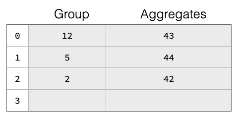
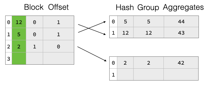
Both chaining and linear probing will degrade in theoretical lookup performance from O(1) to O(n) wrt hash table size if there are too many collisions, i.e. too many groups hashing to the same hash table entry. A common solution to this problem is to resize the hash table once the “fill ratio” exceeds some threshold, e.g. 75% is the default for Java’s HashMap. This is particularly important as we do not know the amount of groups in the result before starting the aggregation. Neither do we assume to know the amount of rows in the input table. We thus start with a fairly small hash table and resize it once the fill ratio exceeds a threshold. The basic hash table structure is shown in the figure below, the table has four slots 0-4. There are already three groups in the table, with group keys 12, 5 and 2. Each group has aggregate values (e.g. from a SUM) of 43 etc.
A big challenge with the resize of a partially filled hash table after the resize, all the groups are in the wrong place and we would have to move everything, which will be very expensive.
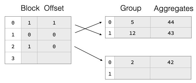
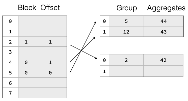
To support resize efficiently, we have implemented a two-part aggregate hash table consisting of a separately-allocated pointer array which points into payload blocks that contain grouping values and aggregate states for each group. The pointers are not actual pointers but symbolic, they refer to a block ID and a row offset within said block. This is shown in the figure above, the hash table entries are split over two payload blocks. On resize, we throw away the pointer array and allocate a bigger one. Then, we read all payload blocks again, hash the group values, and re-insert pointers to them into the new pointer array. The group data thus remains unchanged, which greatly reduces the cost of resizing the hash table. This can be seen in the figure below, where we double the pointer array size but the payload blocks remain unchanged.
The naive two-part hash table design would require a re-hashing of all group values on resize, which can be quite expensive especially for string values. To speed this up, we also write the raw hash of the group values to the payload blocks for every group. Then, during resize, we don’t have to re-hash the groups but can just read them from the payload blocks, compute the new offset into the pointer array, and insert there.
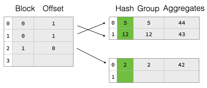
The two-part hash table has a big drawback when looking up entries: There is no ordering between the pointer array and the group entries in the payload blocks. Hence, following the pointer creates random access in the memory hierarchy. This will lead to unnecessary stalls in the computation. To mitigate this issue, we extend the memory layout of the pointer array to include some (1 or 2) bytes from the group hash in addition to the pointer to the payload value. This way, linear probing can first compare the hash bits in the pointer array with the current group hash and decide whether it’s worth following the payload pointer or not. This can potentially continue for every group in the pointer chain. Only when the hash bits match we have to actually follow the pointer and compare the actual groups. This optimization greatly reduces the amount of times the pointer to the payload blocks has to be followed and thereby reduces the amount of random accesses into memory which are directly related to overall performance. It has the nice side-effect of also greatly reducing full group comparisons which can also be expensive, e.g. when aggregating on groups that contain strings.
Another (smaller) optimization here concerns the width of the pointer array entries. For small hash tables with few entries, we do not need many bits to encode the payload block offset pointers. DuckDB supports both 4 byte and 8 byte pointer array entries.
For most aggregate queries, the vast majority of query processing time is spent looking up hash table entries, which is why it’s worth spending time on optimizing them. If you’re curious, the code for all this is in the DuckDB repo, aggregate_hashtable.cpp. There is another optimization for when we know that there are only a few distinct groups from column statistics, the perfect hash aggregate, but that’s for another post. But we’re not done here just yet.
Parallel Aggregation
While we now have an aggregate hash table design that should do fairly well for grouped aggregations, we still have not considered the fact that DuckDB automatically parallelizes all queries to use multiple hardware threads (“CPUs”). How does parallelism work together with hash tables? In general, the answer is unfortunately: “Badly”. Hash tables are delicate structures that don’t handle parallel modifications well. For example, imagine one thread would want to resize the hash table while another wants to add some new group data to it. Or how should we handle multiple threads inserting new groups at the same time for the same entry? One could use locks to make sure that only one thread at a time is using the table, but this would mostly defeat parallelizing the query. There has been plenty of research into concurrency-friendly hash tables but the short summary is that it’s still an open issue.
It is possible to let each thread read data from downstream operators and build individual, local hash tables and merge those together later from a single thread. This works quite nicely if there are few groups like in the example at the top of this post. If there are few groups, a single thread can merge many thread-local hash tables without creating a bottleneck. However, it’s entirely possible there are as many groups as there are input rows, for this tends to happen a lot when someone groups on a column that would be a candidate for a primary key, e.g. observation_number, timestamp etc. What is thus needed is a parallel merge of the parallel hash tables. We adopt a method from Leis et al.: Each thread builds not one, but multiple partitioned hash tables based on a radix-partitioning on the group hash.
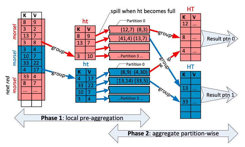
The key observation here is that if two groups have a different hash value, they cannot possibly be the same. Because of this property, it is possible to use the hash values to create fully independent partitions of the groups without requiring any communication between threads as long as all the threads use the same partitioning scheme (see Phase 1 in the above diagram).
After all the local hash tables have been constructed, we assign individual partitions to each worker thread and merge the hash tables within that partition together (Phase 2). Because the partitions were created using the radix partitioning scheme on the hash, all worker threads can independently merge the hash tables within their respective partitions. The result is correct because each group goes into a single partition and that partition only.
One interesting detail is that we never need to build a final (possibly giant) hash table that holds all the groups because the radix group partitioning ensures that each group is localized to a partition.
There are two additional optimizations for the parallel partitioned hash table strategy: 1) We only start partitioning once a single thread’s aggregate hash table exceeds a fixed limit of entries, currently set to 10 000 rows. This is because using a partitioned hash table is not free. For every row added, we have to figure out which partition it should go into, and we have to merge everything back together at the end. For this reason, we will not start partitioning until the parallelization benefit outweighs the cost. Since the partitioning decision is individual to each thread, it may well be possible only some threads start partitioning. If that is the case, we will need to partition the hash tables of the threads that have not done so before starting merging them. This is a fully thread-local operation however and does not interfere with parallelism. 2) We will stop adding values to a hash table once its pointer array exceeds a certain threshold. Every thread then builds multiple sets of potentially partitioned hash tables. This is because we do not want the pointer array to become arbitrarily large. While this potentially creates duplicate entries for the same group in multiple hash tables, this is not problematic because we merge them all later anyway. This optimization works particularly well on data sets that have many distinct groups, but have group values that are clustered in the input in some manner. For example, when grouping by day in a data set that is ordered on date.
There are some kinds of aggregates which cannot use the parallel and partitioned hash table approach. While it is trivial to parallelize a sum, because the sum of the overall result is just the sum of the individual results, this is fairly impossible for computations like median, which DuckDB also supports. Also for this reason, DuckDB also supports approx_quantile, which is parallelizable.
Experiments
Putting all this together, it’s now time for some performance experiments. We will compare DuckDB’s aggregation operator as described above with the same operator in various Python data wrangling libraries. The other contenders are Pandas, Polars and Arrow. Those are chosen since they can all execute an aggregation operator on Pandas DataFrames without converting into some other storage format first, just like DuckDB.
For our benchmarks, we generate a synthetic dataset with a pre-defined number of groups over two integer columns and some random integer data to aggregate. The entire dataset is shuffled before the experiments to prevent taking advantage of the clustered nature of the synthetically generated data. For each group, we compute two aggregates, sum of the data column and a simple count. The SQL version of this aggregation would be SELECT g1, g2, sum(d), count(*) FROM dft GROUP BY g1, g2 LIMIT 1;. In the experiments below, we vary the dataset size and the amount of groups in them. This should nicely show the scaling behavior of the aggregation.
Because we are not interested in measuring the result set materialization time which would be significant for millions of groups, we follow the aggregation with an operator that only retrieves the first row. This does not change the complexity of the aggregation at all, since it needs to collect all data before producing even the first result row, since there might be data in the very last input data row that changes results for the first result. Of course this would be fairly unrealistic in practice, but it should nicely isolate the behavior of the aggregation operator only, since a head(1) operation on three columns should be fairly cheap and constant in execution time.

We measure the elapsed wall clock time required to complete each aggregation. To account for minor variation, we repeat each measurement three times and report the median time required. All experiments were run on a 2021 MacBook Pro with a ten-core M1 Max processor and 64 GB of RAM. Our data generation benchmark script is available online and we invite interested readers to re-run the experiment on their machines.

Now let’s discuss some results. We start with varying the amount of rows in the table between one million and 100 millions. We repeat the experiment for both a fixed (small) group count of 1000 and when the amount of groups is equal to the amount of rows. Results are plotted as a log-log plot, we can see how DuckDB consistently outperforms the other systems, with the single-threaded Pandas being slowest, Polars and Arrow being generally similar.

For the next experiment, we fix the amount of rows at 100M (the largest size we experimented with) and show the full behavior when increasing the group size. We can see again how DuckDB consistently exhibits good scaling behavior when increasing group size, because it can effectively parallelize all phases of aggregation as outlined above. If you are interested in how we generated those plots, the plotting script is available, too.
Conclusion
Data analysis pipelines using mostly aggregation spend the vast majority of their execution time in the aggregate hash table, which is why it is worth spending an ungodly amount of human time optimizing them. We have some ideas for future work on this, for example we would like to extend our work when comparing sorting keys to comparing groups in the aggregate hash table. We also would like to add capabilities of dynamically choosing the amount of partitions a thread uses based on dynamic observation of the created hash table, e.g. if partitions are imbalanced we could use more bits to do so. Another large area of future work is to make our aggregate hash table work with out-of-core operations, where an individual hash table no longer fits in memory, this is particularly problematic when merging. And of course there are always opportunities to fine-tune an aggregation operator, and we are continuously improving DuckDBs aggregation operator.
If you want to work on cutting edge data engineering like this that will be used by thousands of people, consider contributing to DuckDB or join us at DuckDB Labs in Amsterdam!